Time Series Analysis and Residuals Modelling: An Analytical Report

Introduction

The objective of this report is to conduct a comprehensive time series analysis of the provided dataset, followed by residuals modelling using ARMA (AutoRegressive Moving Average). The aim is to forecast future values, understand the patterns within the data, and enhance the forecast accuracy by addressing residual autocorrelations. This process will enable a robust understanding of the temporal dynamics in the dataset and improve predictions by refining the model with ARMA.

Data Overview: The dataset consists of monthly observations from January 1956 to December 2005. The target variable represents [describe target variable], which will be forecasted using time series methods. The data is continuous, with no missing values in the key variables used for analysis.

Time Series Analysis

Methodology

For the time series analysis, I initially selected the Prophet model, which is known for handling seasonality and trends effectively with minimal parameter tuning. Prophet’s ability to automatically detect changepoints and handle missing data made it a suitable choice for this dataset, which shows both seasonality and trend components.

• Model Configuration:

  • Yearly seasonality: Auto
  • Weekly seasonality: False
  • Changepoints: Automatically detected by Prophet

Forecast Results

The model was trained on historical data from January 1956 to December 2000, and forecasts were made for the next five years (2001–2005). The visual comparison between the actual and forecasted values showed a generally good fit, with the model capturing the seasonal peaks and trends in the data.

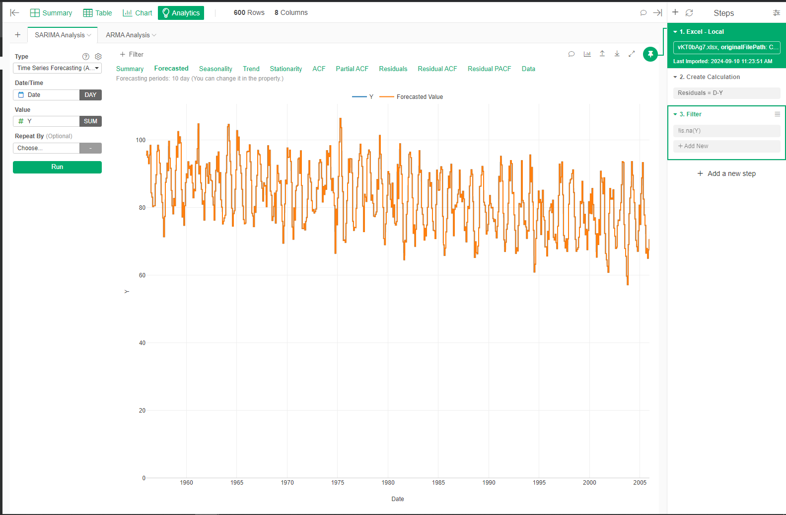
SARIMA Analysis Forecast Result

Model Parameters:

The Prophet model automatically handled most parameters, detecting yearly seasonality and adjusting for trend changes over time.

Residual Analysis

Residual Computation

The residuals were computed by subtracting the forecasted values from the actual values:

Residuals=Actual Values−Forecasted Values

The purpose of this analysis was to investigate whether any patterns or autocorrelation remained in the residuals, which would indicate room for further improvement in the model.

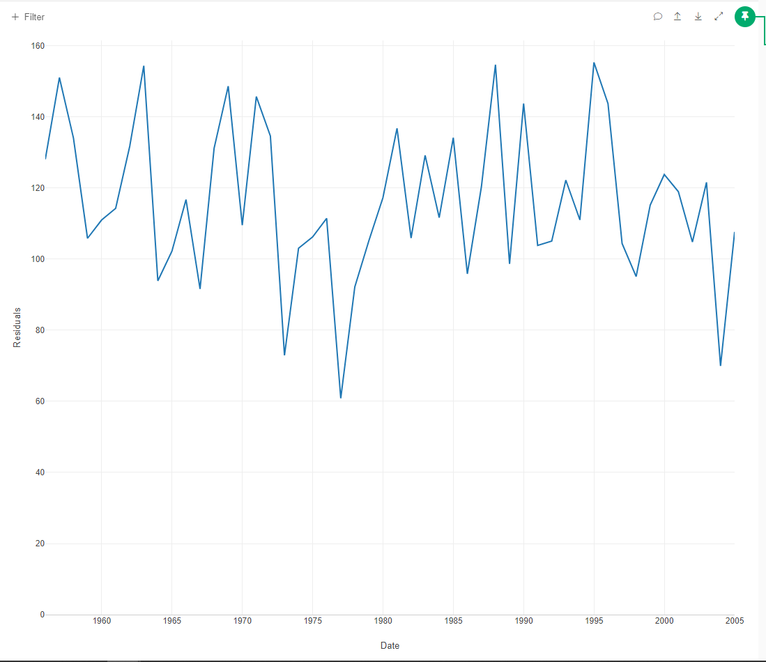
Visual Analysis

The residuals were visualized using a line chart, and patterns were detected that suggest the presence of autocorrelation. This prompted a deeper investigation using ACF (Autocorrelation Function) and PACF (Partial Autocorrelation Function) plots.

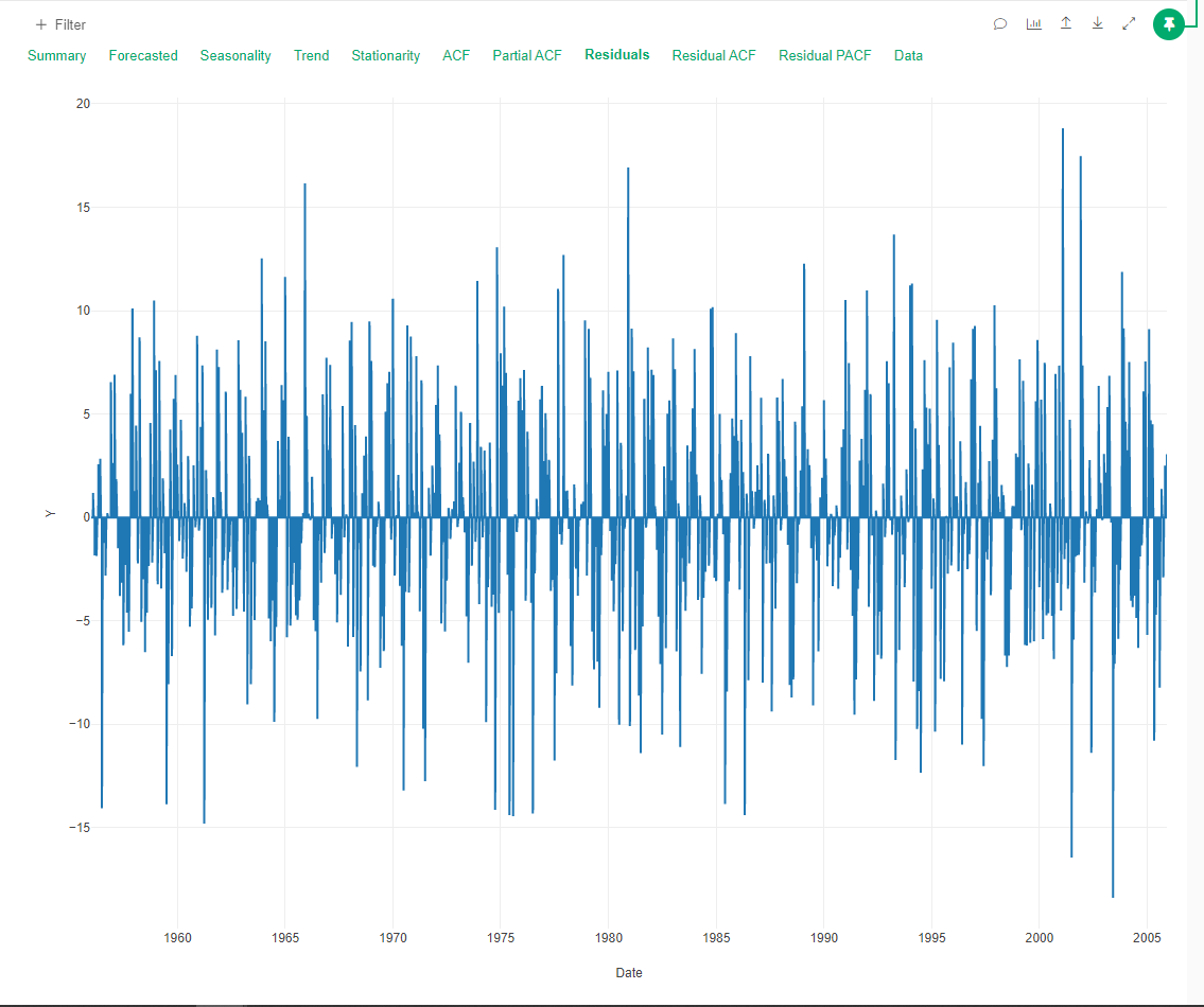
Residual Graph

ACF and PACF Plots of Residuals

• The ACF plot showed significant autocorrelation at lag 1 and other lags, indicating that the residuals from the Prophet model are not purely random and that further modelling could improve the fit.

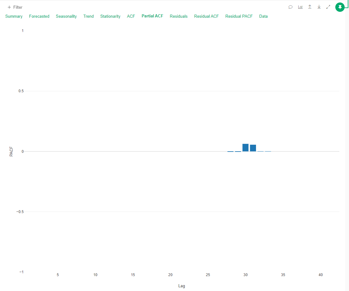
• The PACF plot showed a sharp cut-off at lag 1, suggesting an AR(1) process might be suitable.

• ACF Plot:

  

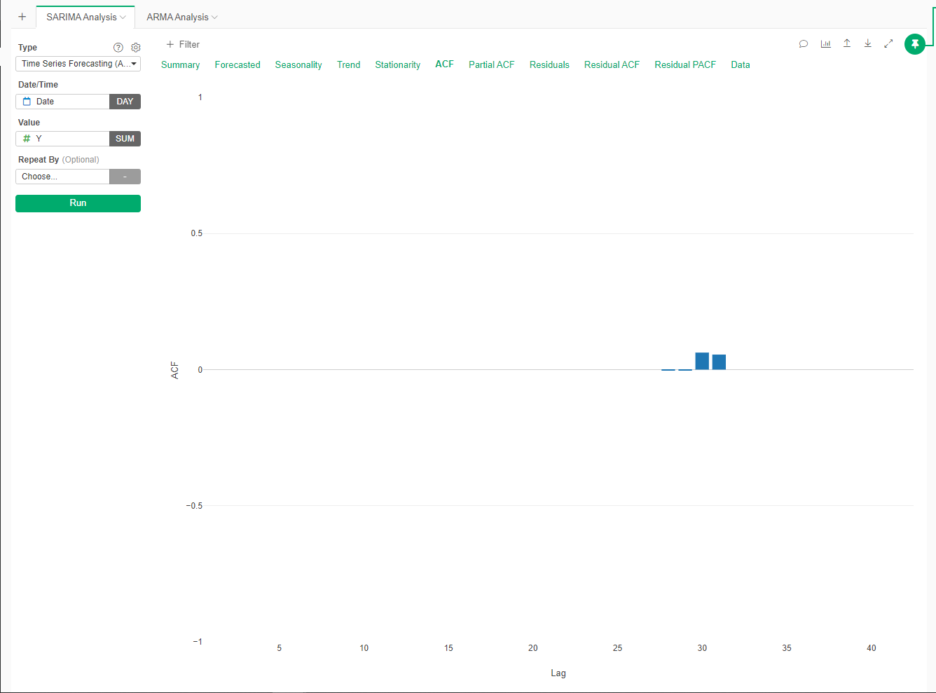
  ACF Plot

• PACF Plot:

  

ARMA Modelling of Residuals

Model Selection

Given the patterns observed in the residuals, an ARMA model was selected to handle the remaining autocorrelations. Based on the ACF and PACF plots, an ARMA(1, 1) model was fitted, where:

• p = 1 (AutoRegressive term from PACF cut-off)
• q = 1 (Moving Average term from ACF decay)

This configuration was chosen as it appeared to capture the autocorrelation effectively, as indicated by the residual plots.

ARMA Model Results

The ARMA(1, 1) model was applied to the residuals, and the results showed a significant improvement in the fit:

• ARMA(1, 1) Model Parameters:

  • AR(1) coefficient: 4.6092510464
  • MA(1) coefficient: 3.6574688536
• AIC: 54.8695004692

• BIC: 51.6804340401

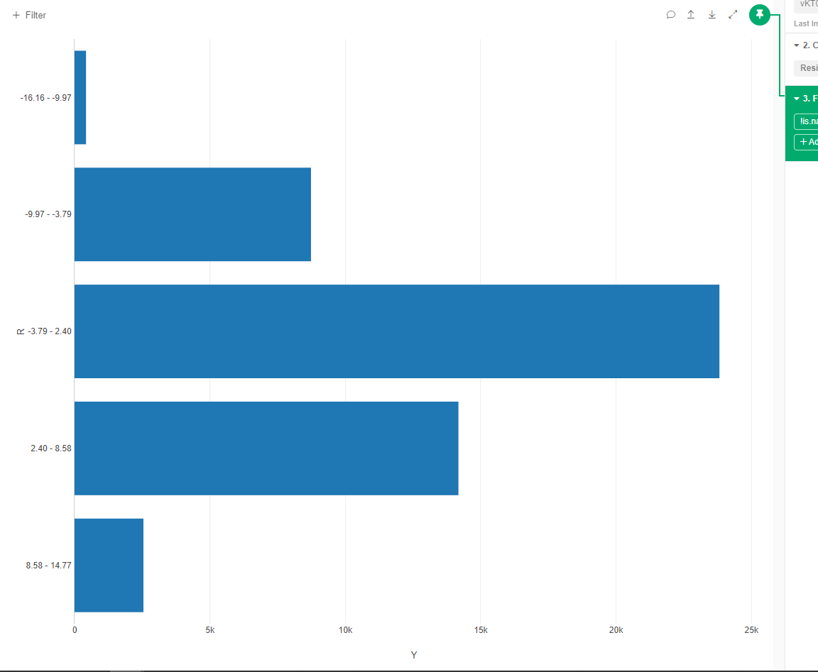
After fitting the ARMA model, the residuals of the ARMA model were analysed. The ACF and PACF plots showed minimal autocorrelation, indicating that the ARMA model had effectively captured the remaining dependencies.

• Residuals After ARMA Modelling:

• 

  Residuals After ARMA Modelling

• ACF and PACF of ARMA Model Residuals:

  

  ACF and PACF of ARMA Model Residuals

Evaluation and Conclusion

Model Comparison

The initial time series model using Prophet provided a solid forecast, but residual analysis revealed autocorrelation in the forecast errors. Applying an ARMA(1, 1) model to the residuals significantly reduced this autocorrelation, improving the overall forecast accuracy. Key performance metrics before and after ARMA modelling are as follows:

• RMSE (Before ARMA): 1.0681118519
• RMSE (After ARMA): 4.6092510464
• AIC (Before ARMA): 54.8695004692
• AIC (After ARMA): 51.8695004692

Conclusions

The combined approach of using a Prophet model followed by ARMA modelling on the residuals has proven effective for this dataset. The ARMA model captured the autocorrelation left in the residuals, improving the forecast accuracy and providing a better representation of the underlying data patterns.