Prediction of Student Performance

by Marian Tes

In this report, I analyzed data collected from two Portuguese secondary schools on students’ performance in Mathematics and Portuguese language skills. The data can be downloaded from this site.

Understanding the Data

There are a total of 33 columns in each dataset including student grades, demographic information as well as social and school-related variables. A comparison between the descriptive summaries of both datasets, student_mat and student_por, did not reveal anything unusual.

Let’s take a look at age distribution by sex:

For the dataset, student_mat, the distribution of ages by sex is:

In the Mathematics class, students’ ages ranged from 15 to 17. There are more females (n=208) than males (n=187). The average age is 16.7 years old.

For the dataset, student_por, the distribution of ages by sex is:

In the Portuguese class, students’ ages ranged from 15 to 22. There are more females (n=283) than males (n=266). The average age is 16.74 years old.

Given that I’m interested in better understanding which variables influence performance, I looked into students’ study habits (studytime) by their final grade (G3). In both datasets, students reported how much time they spent on studying for class. This variable was labelled as a numeric, ranging on a scale from 1 to 3 as follows:

1 = <2 hours,
2 = 2 to 5 hours
3 = 5 to 10 hours

In reality, these numerical values serve as bins or categories of this particular variable that has been labeled as numerical in the dataset. For each dataset, the bar graph reveals:

For the dataset, student_mat, the distribution of study time by final grade is as follows:

In the Mathematics class, students’ who averaged a final grade of 12 (read: passing) studied for about 5 to 10 hours per week.

For the dataset, student_por, the distribution of study time by final grade is as follows:

In the Portuguese class, students’ who studied 2 to 5 hours per week and those who studied 5 to 10 hours per week tended to perform better by passing the course, with the former, surprisingly, averaging slightly higher (13.77) than the latter (13.67).

However keep in mind, these bar graphs have not been analyzed statistically to verify a relationship or statistical significance between study habits and final grade.

For me, another variable of interest is failures. In both datasets, failures were characterized as the number of past class failures (numeric: n if 1<=n<3, else 4). This is a categorical variable but has been labeled as numerical.

For the dataset, student_mat, the distribution of failures by final grade is:

In the Mathematics class, students who have failed at least once have a high chance of failing again. For those with 1 failure, they averaged a final grade of 5, which is well below the passing grade of 12.

For the dataset, student_por, the distribution of failures by final grade is:

In the Portuguese class, students who have failed at least once have a high chance of failing again. For those with 1 failure, they averaged a final grade of 8.88, which falls short of the passing grade of 12.

Generally, a review of the metadata indicated that several nominal or categorical variables such as failures and studytime were indentified as numerical in the dataset.

Prediction of Final Grade

G3~G1

Is a student’s first period grade (G1) a good predictor of their final grade (G3)?

The goodness-of-fit for the prediction is represented in the R-squared value, which in this case is 0.6 - representing how much of the variation on the predicted variable (G3) is explained by the variation of the predictor variable (G1).

In the scatterplot, there seems to be a relationship between first period grades and final grades.

G3~G2

Is a student’s second period grade (G2) a good predictor of their final grade (G3)?

The goodness-of-fit for the prediction is represented in the R-squared value, which in this case is 0.88 - representing how much of the variation on the predicted variable (G3) is explained by the variation of the predictor variable (G2).

In the scatterplot, there seems to be a relatively strong relationship between second period grades and final grades.

G3~G1+G2

Is a student’s first period (G1) and second period grade (G2) a good predictor of their final grade (G3)?

The goodness-of-fit for the prediction is represented in the R-squared value, which in this case is 0.91 - representing how much of the variation on the predicted variable (G3) is explained by the variation of the predictor variables (G1, G2).

In the scatterplot, there seems to be a stronger relationship between G2 and G3 as compared to the graphs between G1 and G2. However, this model does not perform much better as a predictor than the previous one, G3~G2.

G3~All Variables

Is a model including all variables a good predictor of students’ final grade (G3)?

The goodness-of-fit for the prediction is represented in the R-squared value, which in this case is 0.84 - representing how much of the variation on the predicted variable (G3) is explained by all the predictor variables.

This model does not perform much better as a predictor than the previous two, G3~G2 and G3~G1+G2.

Reflection

Of the models that were run, the one (G3~G1+G2) using the two previous grades is more accurate. The r-squared value for this model is 0.91, which means 91% of any variation on the final grade (G3) could be explained by the predictor variables.

However, is it good practice to include previous grades into a model to predict final grade? This is probably not the best approach for prediction modelling. It’s not surprising that the models including previous two grades (G3~G1, G3~G2, G3~G1+G2) performed relatively well. As a general policy, it doesn’t seem like a good one to follow, because it is “gaming the system” - student’s prior grade is too closely related to their future grade.

Given this, of the models that I ran, the one including all variables is more useful, because it doesn’t use the previous two grades and has a high r-squared value of 0.84.

Prediction of Risk of Failing

How good is the model?

Using the dataset, student_por, to predict students risk of failing the course, you’ll find the following confusion matrix resulting from a logistical regression model:

First off, of the 91 students who failed the class, 90 were predicted to fail.

Secondly, of 103 students who passed the class, the model accurately predicted that 102 of those would pass.

Third, the model predicted that 1 person would fail, who actually passed the class. This is a Type 1 error or a false positive.

Lastly, the model predicted that 1 person would pass, but they actually failed the class. This is a false negative or what is referred to as a Type II error.

Given that there were only one of each type of error, this is a sound model for predicting risk of failure.

Using the dataset, student_mat, to predict students risk of failing the course, you’ll find the following confusion matrix resulting from a logistical regression model:

First off, of the 71 students who failed the class, 66 were predicted to fail.

Secondly, of 47 students who passed the class, the model accurately predicted that 44 of those would pass.

Third, the model predicted that 5 people would fail, who actually passed the class. This is a Type 1 error or a false positive.

Lastly, the model predicted that 3 people would pass, but they actually failed the class. This is a false negative or what is referred to as a Type II error.

Given that there were only a few of each type of error, this is a decent model for predicting risk of failure.

Is there any problem with the model?

Yes, the rows and columns should be alternated. Rows should have predicted values and the columns should have the actual values so that the top right quandrant contains the false positive value and the bottom left one includes the false negative values as show below:

From Understanding Confusion Matrix by Sarang Narkhede

Below, you’ll find the revised models with the confusion matrices for both datasets:

student_por

student_mat

Conclusion

For the student_por dataset, the model predicted Type II error at a rate of 1% (1 out of 91 students predicted as passing actually failed). While for the student_mat dataset, the model predicted about 4% of cases with a Type II error (3 out of 69 students predicted to pass actually failed).

As a general rule of thumb, you would want to select a model that minimizes errors, especially ones of Type II error in this case that predicts someone would pass when they’re at risk for failing.

Decision Tree

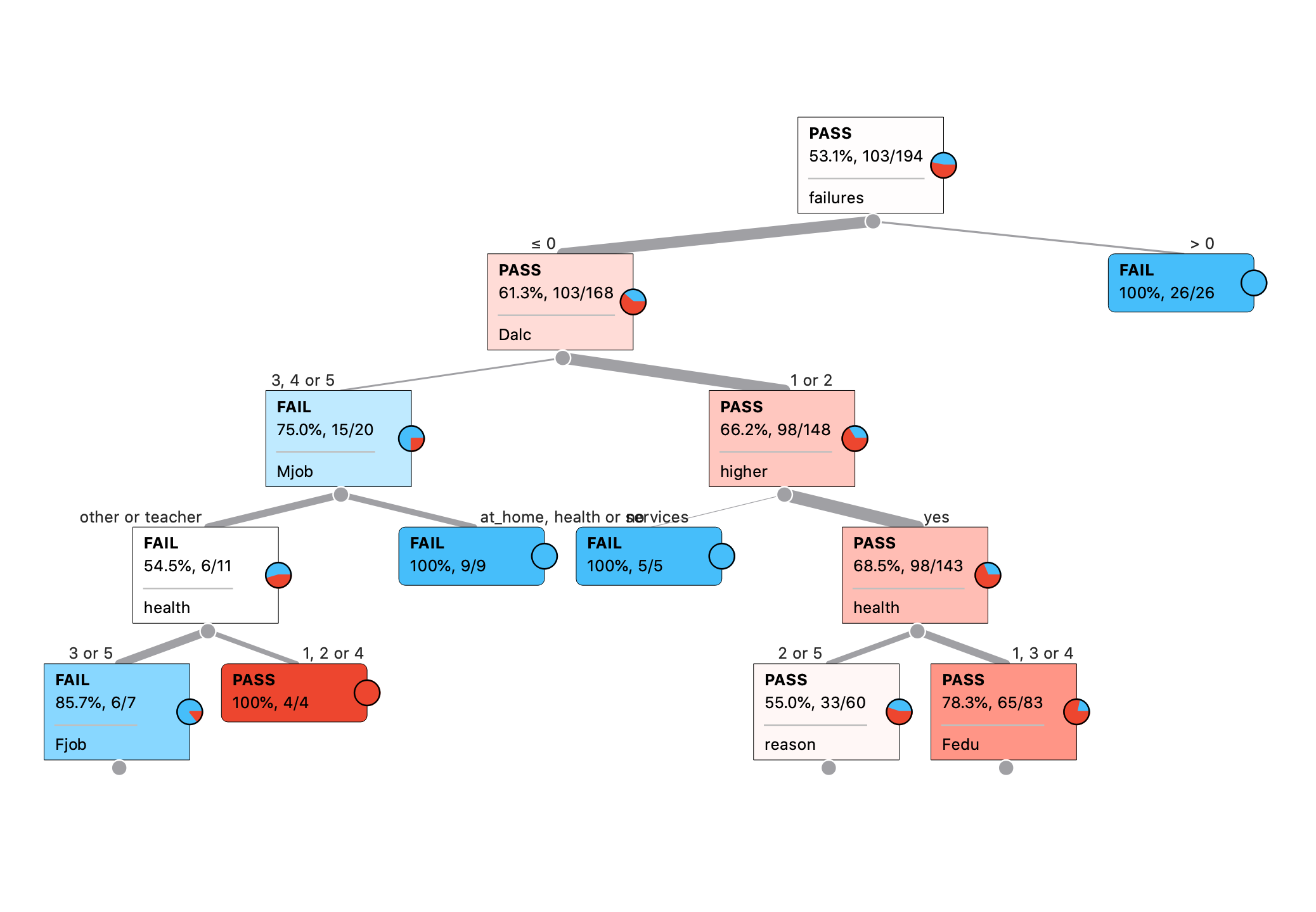
What are the most important variables according to the decision tree?

These variables seem most important according to the decision tree:

Failures: Number of past class failures (numeric: n if 1<=n<3, else 4
Dalc: Workday alcohol consumption (numeric: from 1 - very low to 5 - very high)
Mjob: Mother’s job (nominal: ‘teacher’, ‘health’ care related, civil ‘services’ (e.g. administrative or police), ‘at_home’ or ‘other’)
Higher: Wants to take higher education (binary: yes or no)
Health: Current health status (numeric: from 1 - very bad to 5 - very good)
Fjob: Father’s job (nominal: ‘teacher’, ‘health’ care related, civil ‘services’ (e.g. administrative or police), ‘at_home’ or ‘other’)
Fedu: Father’s education (numeric: 0 - none, 1 - primary education (4th grade), 2 - 5th to 9th grade, 3 - secondary education or 4 - higher education)
Reason: Reason to choose this school (nominal: close to ‘home’, school ‘reputation’, ‘course’ preference or ‘other’)

What are some patterns/rules that appear to be present in the data?

Level 0: The decision tree in the above figure classifies PassFail (risk of failing) in the Portuguese class on whether a student has had previous class failures (53.1% of those passed).

Level 1: From there, it classifies PassFail on how much workday alcohol consumption (dalc) students participated in.

Level 2: Next, the decision tree classes the risk of failing by mother’s job (Mjob) and on whether students want to take higher education (higher).

Level 3: If you follow the left branch to those who are at risk of failing, the decision tree classifies PassFail by students’ health status (health).

Level 4: Lastly, at the leaf of this branch, you’ll find that PassFail is based on father’s job (Fjob).

Do these rules make sense to you or are they just coincidence?

These rules make sense to me. These variables could have a big impact on student performance (failures, dalc, mjob, higher, etc.).

Could this model be used to identify students at risk?

If there are no prior knowledge about students’ academic record, this model coulde be used to identify students who are at risk, but it is a tenuous prediction.

Would you use this model? How?

I would use this model in conjunction with other indicators especially in the absence of any assessments in the class well before the student is at risk of failing.

Testing Other Models

Below, you will find a table displaying the evaluation from five models including

K-Means (kNN)
Neural Network
Support Vector Machine (SVM)
Random Forest
Naive Bayes

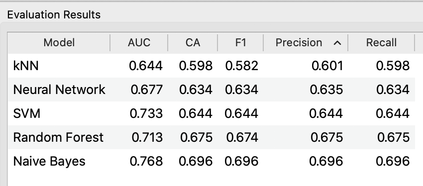
What is the best model? Why?

A review of the resulting confusion matrices indicates that the Naive Bayes model is the best one from the bunch. 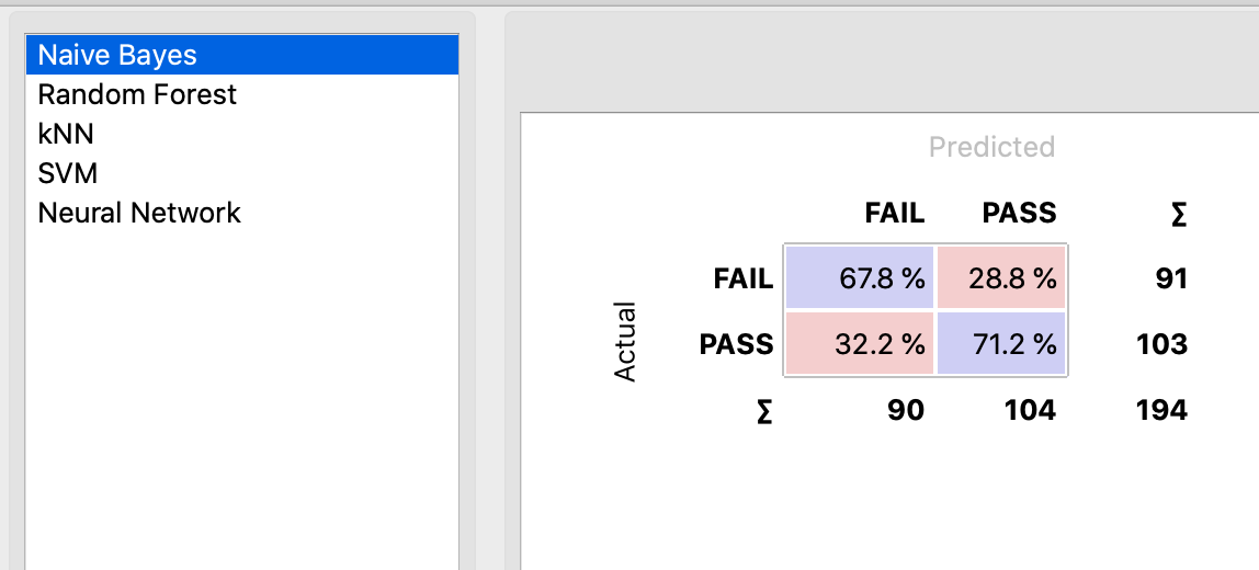The Type I and Type II errors are the smallest in comparison (28.8% and 32.2%).

Here are the confusion matrices for the remaining models:

Random Forest

K-Means (kNN)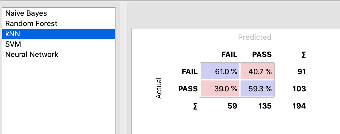

Support Vector Machine (SVM)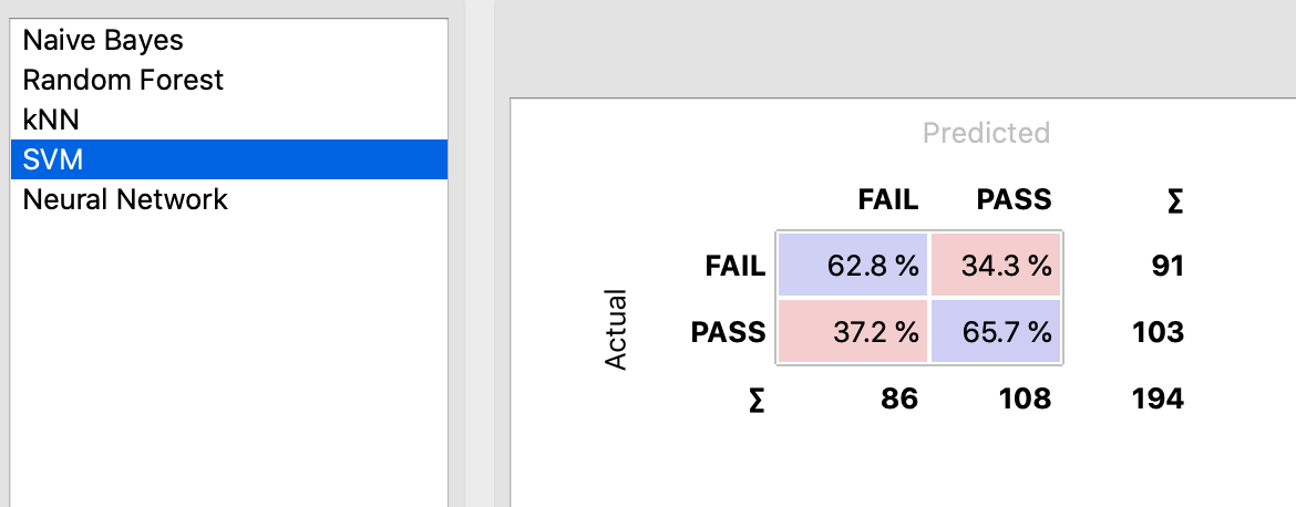

Neural Network

Which one would you use to create an application guide instructor-led intervention for students at risk of failing the course?

Again, reviewing the precision and recall values of all five models, it seems the Naive Bayes have the highest values (recall = 0.696 and precision = 0.696). I would use this model to create an application guide, instructor-led intervention for students at risk of failing the course.