Using forecast (auto.arima) in Exploratory
This note is about using ARIMA for timeseries forcasting in Exploratory. We will use “forecast” package’s auto.arima function through “sweep” package, which provides framework for running timeseries forecast in “tidyverse” way. We will call those packages through Exploratory’s custom model framework.
Overview
Let’s reproduce the forecasting of Nebraska GDP in this article. http://www.business-science.io/code-tools/2017/07/09/sweep-0-1-0.html
Setup
Install dependency packages
Install following 3 packages.
- forecast
- sweep
- timetk
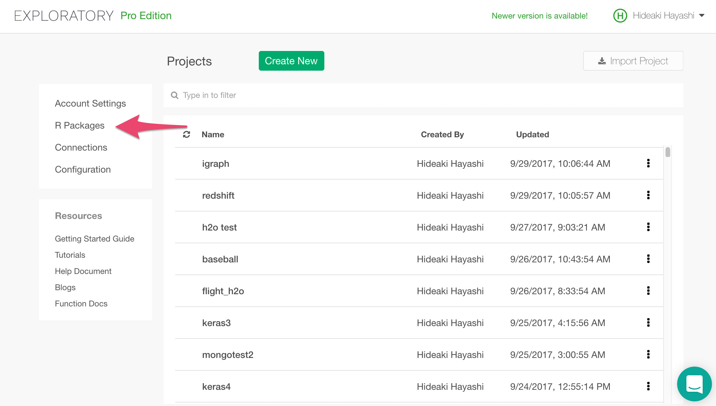
To install a custom package, click R Package menu on project list page.
Then click Install tab, type in package name “forecast”, and click Install button.
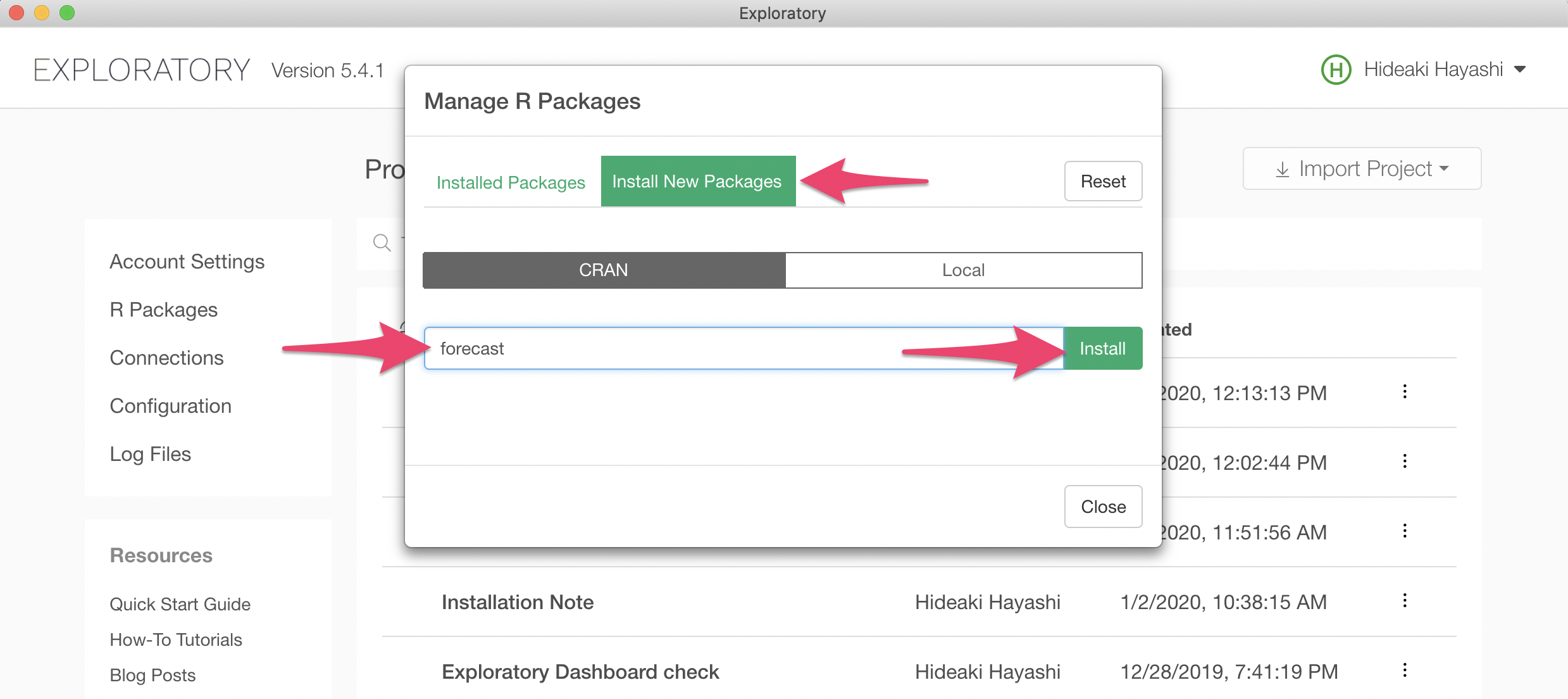
Repeat the same for sweep and timetk packages.
Add forecast::auto.arima as Custom Model
We can add custom model to Exploratory by writing custom R script.
This is a script that adds auto.arima through sweep as a custom model.
library(forecast)   # Most popular forecasting pkg
library(sweep)      # Broom tidiers for forecast pkg
library(timetk)    # Working with time series in R

build_forecast_model <- function(formula, data, freq = 1, periods = 5, ...) {
  training_data <- data

  lhs_cols <- all.vars(lazyeval::f_lhs(formula)) # predicted variable
  rhs_cols <- all.vars(lazyeval::f_rhs(formula)) # date column
  all_cols <- c(lhs_cols, rhs_cols)

  training_data <- training_data[colnames(training_data) %in% all_cols]
  start <- year(training_data[[rhs_cols]][[1]]) # get start year for the following tk_ts()
  training_data_ts <- training_data %>% tk_ts(start=start, freq = freq, silent = TRUE)

  fit_arima <- auto.arima(training_data_ts, ...)

  # return model and periods as one object
  ret <- list(model = fit_arima, periods = periods, value_col = lhs_cols)
  class(ret) <- c("forecast_model")
  ret
}

augment.forecast_model <- function(x, data = NULL, newdata = NULL, ...) {
  fcast <- forecast::forecast(x$model, h = x$periods)
  ret <- sweep::sw_sweep(fcast, timekit_idx = TRUE, rename_index = "date")
  # rename column names of confidence interval so that Exploratory's line chart understands what they are
  colnames(ret)[colnames(ret) == "lo.95"] <- paste0(x$value_col, "_low")
  colnames(ret)[colnames(ret) == "hi.95"] <- paste0(x$value_col, "_high")
  ret
}

glance.forecast_model <- function(x, ...){
  sw_glance(x$model)
}

tidy.forecast_model <- function(x, ...){
  sw_tidy(x$model)
}
Paste the above code in a new Script and save. Here is instruction on creating Script.
Now we are ready to use ARIMA in Exploratory. Let’s use it on the Nebraska GDP data.
Data
Download Data
Download Nebraska GDP data from here as csv file.
Import Data into Exploratory
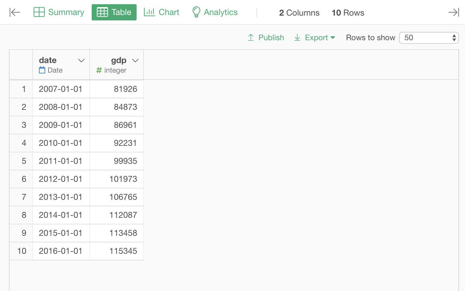
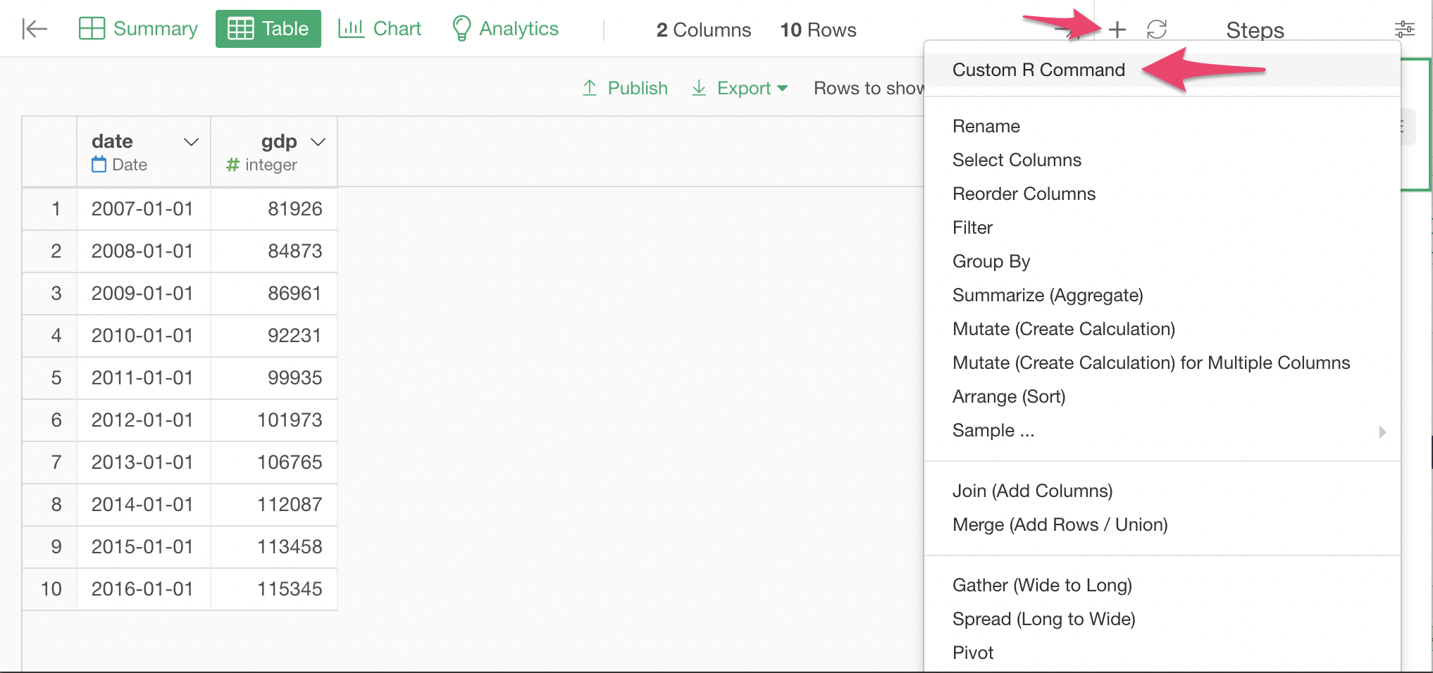
Import downloaded ne_gdp.csv. The imported table on Table View will look like the following.
Build ARIMA Model
Select Custom Command Menu.
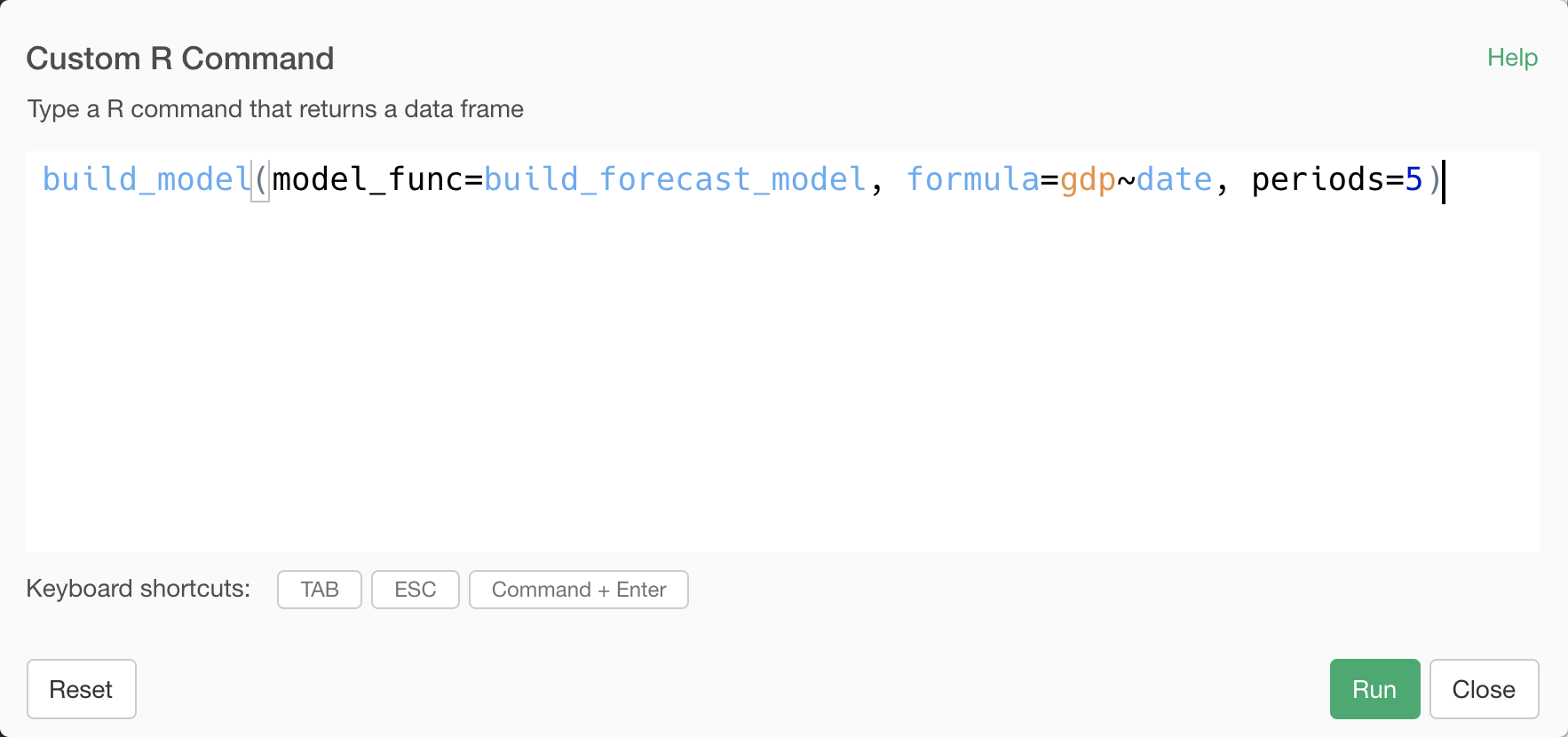
Here is the custom command to create ARIMA model.
build_model(model_func=build_forecast_model, formula=gdp~date, periods=5)Type in the above custom command, and click run button.
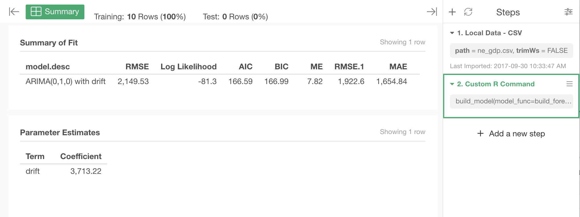
Model is created. Summary of Fit and Parameter Estimates table contents are coming from sweep package’s sw_glance and sw_tidy function.
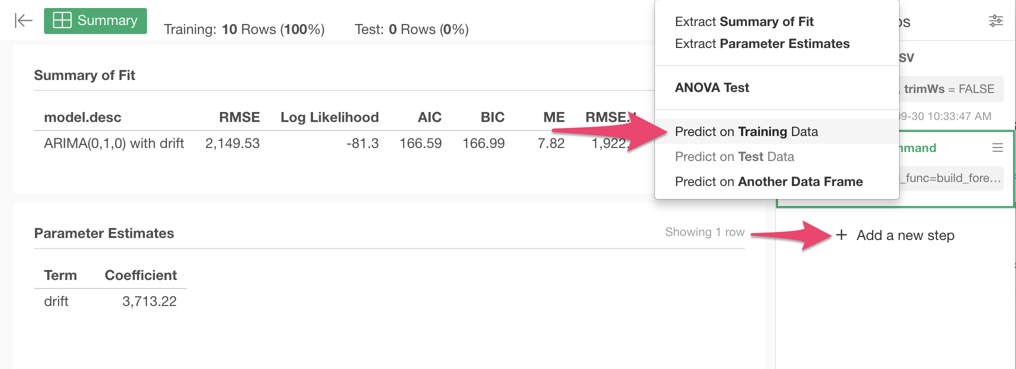
Forecasting
To make a forecast, select “Predict on Training Data” menu.
Click Run button on the Predict Data dialog.
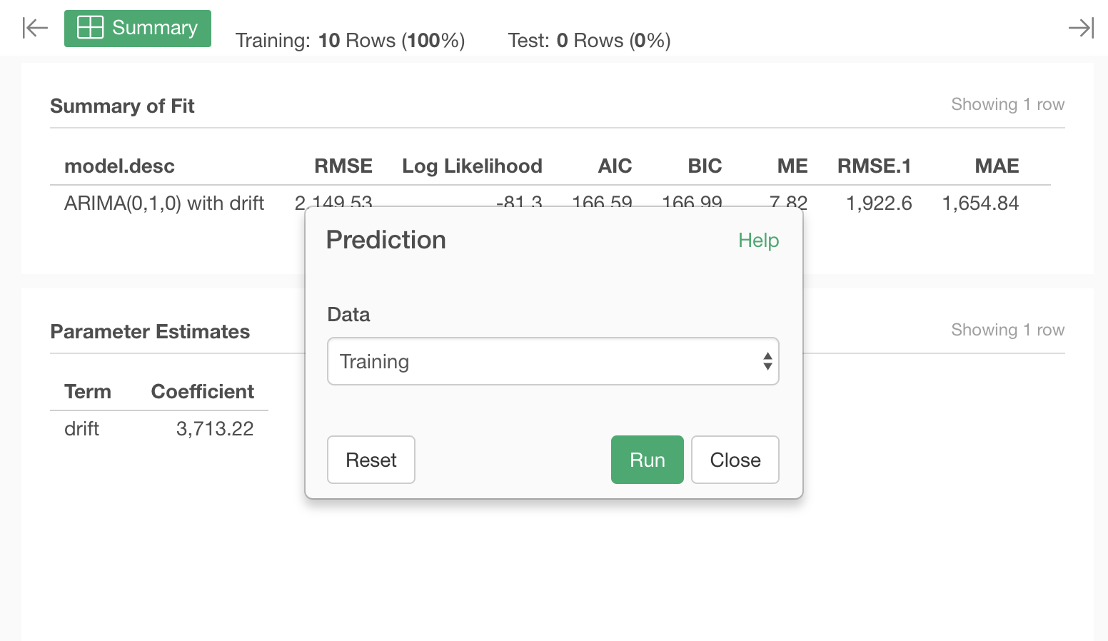
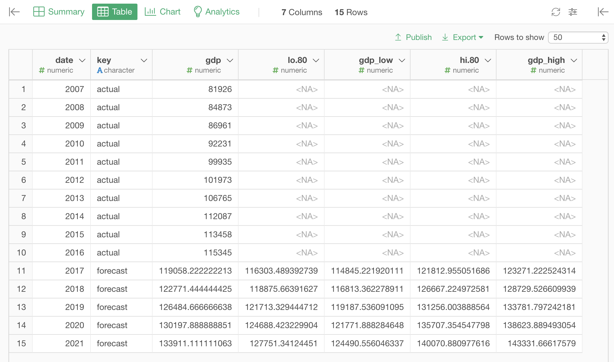
Resulting forecast data will look like this on Table View.
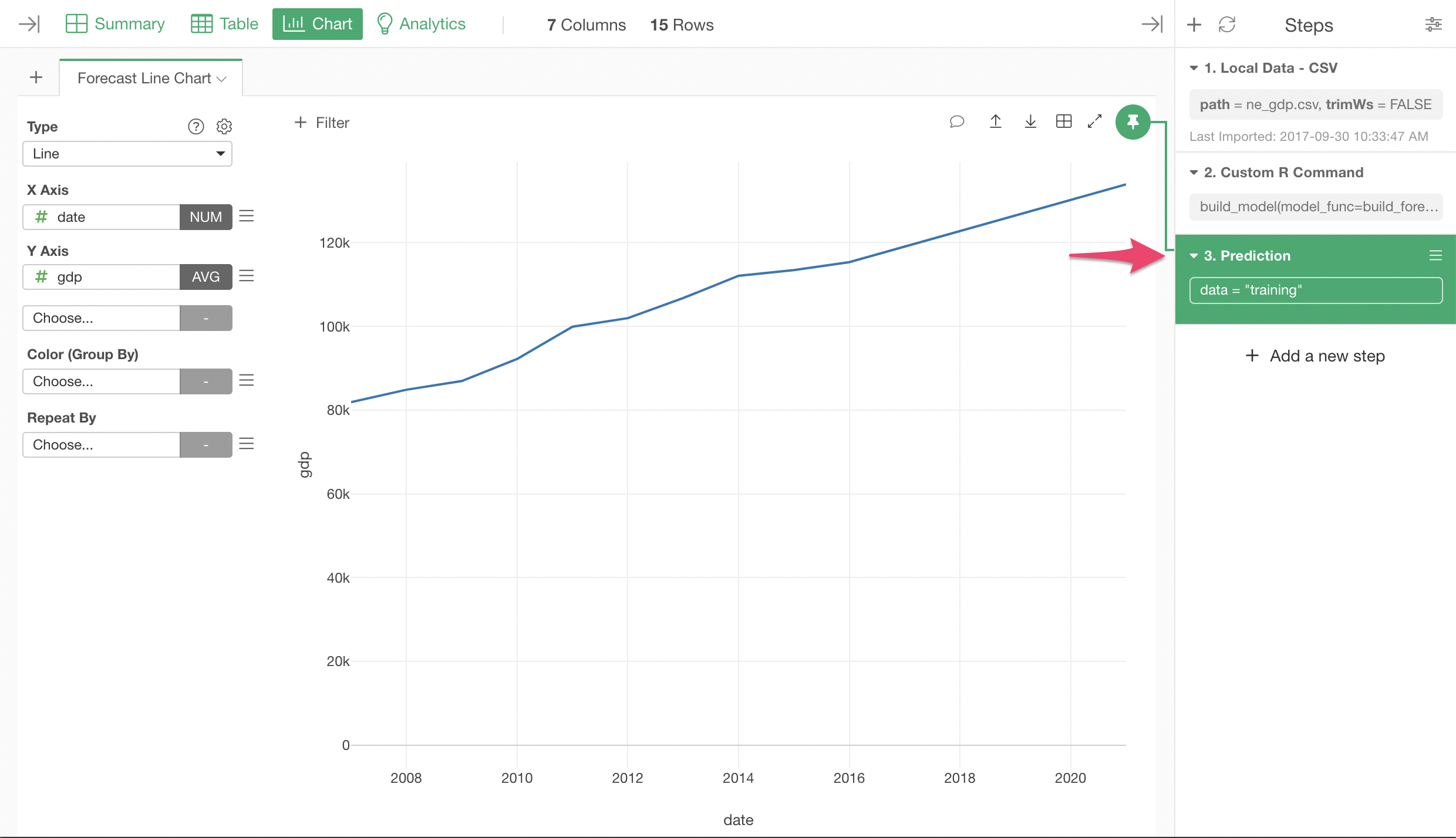
Visualization
Visualize the forecast with Line Chart by selecting X/Y axis columns like the following. Make sure the Chart is pinned to the Prediction step we just added in the previous section.
Let’s display prediction interval. Click Range menu on Y axis.
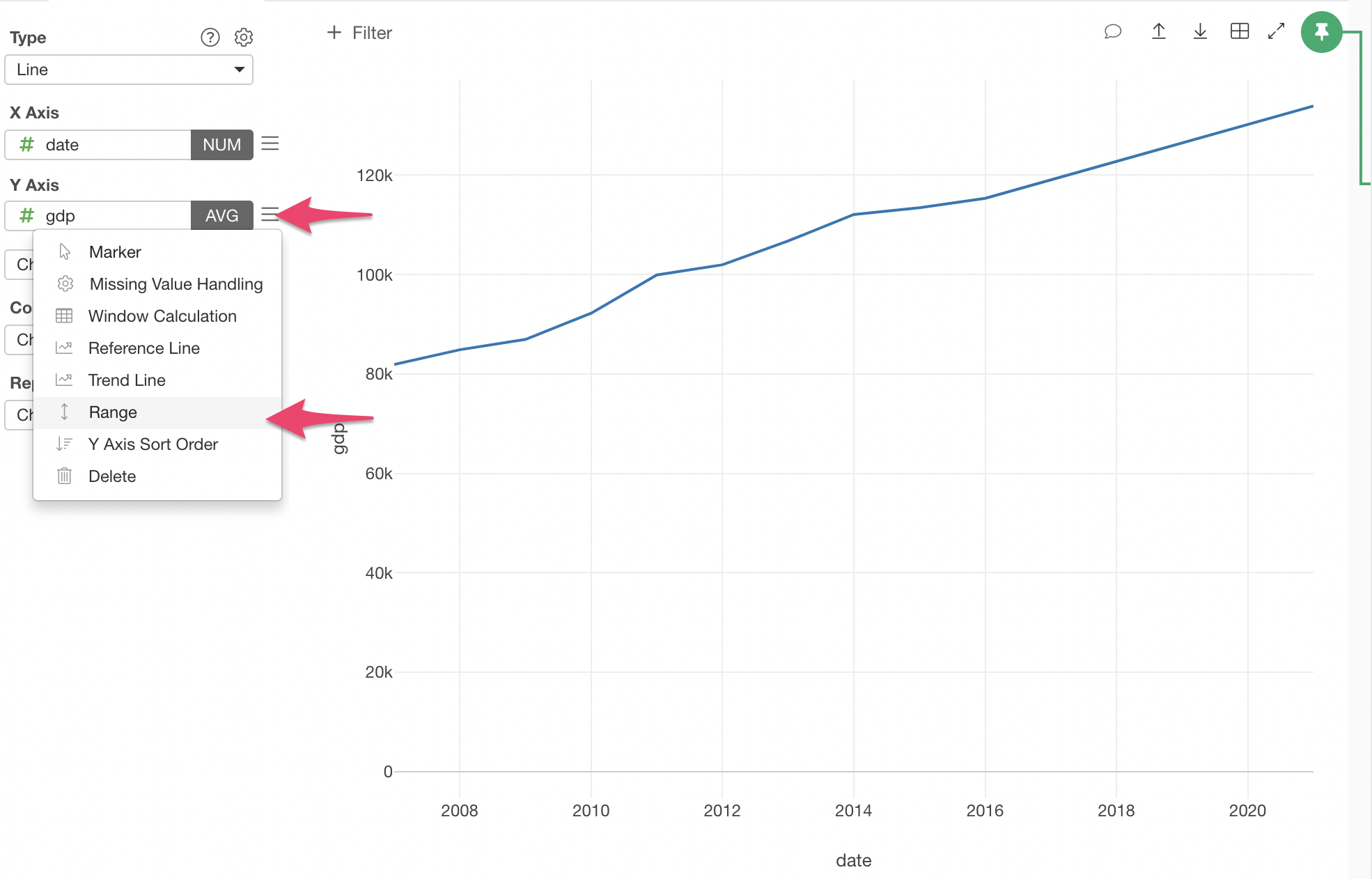
By clicking the checkbox, the columns for range should automatically be set.
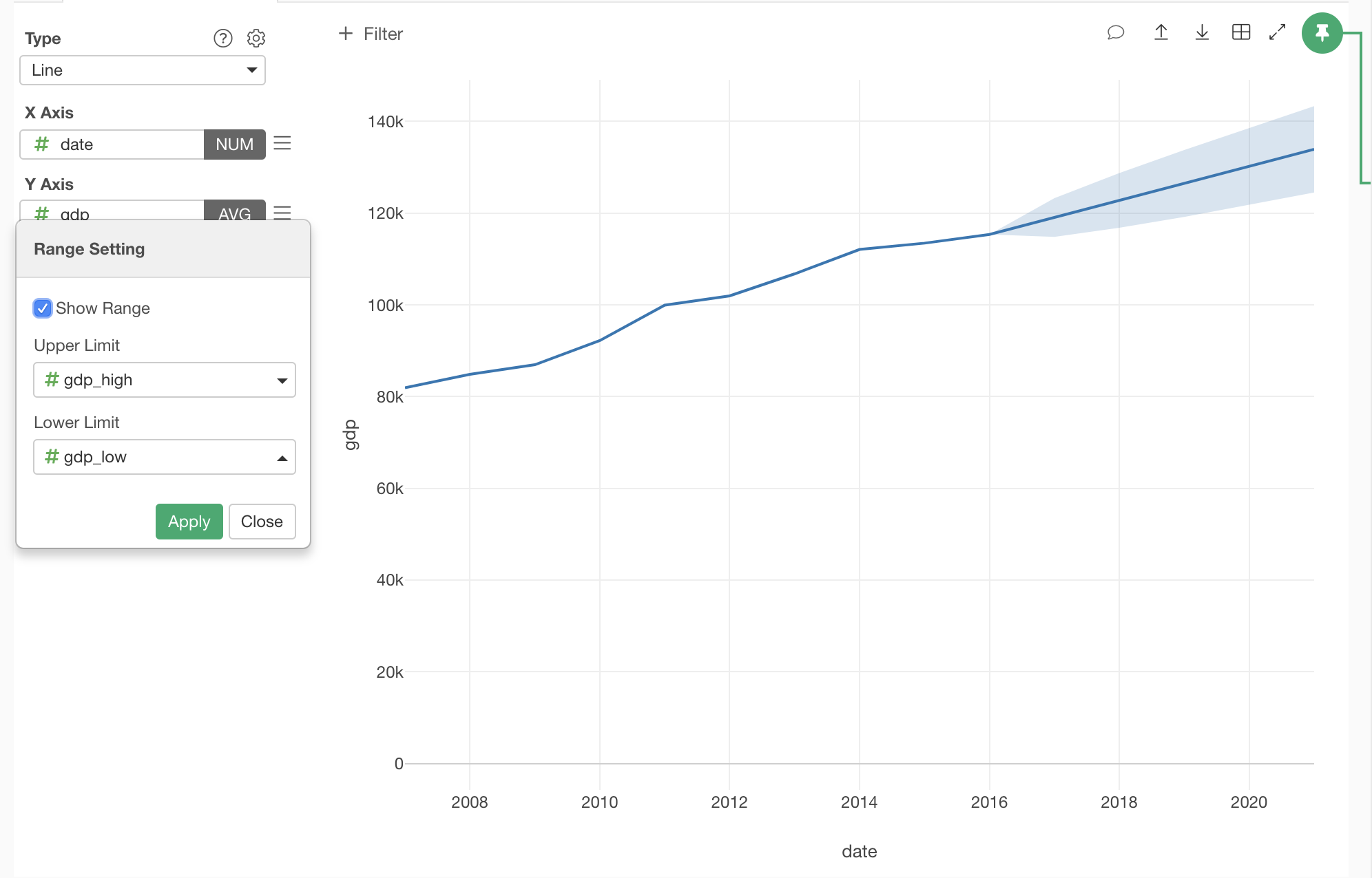
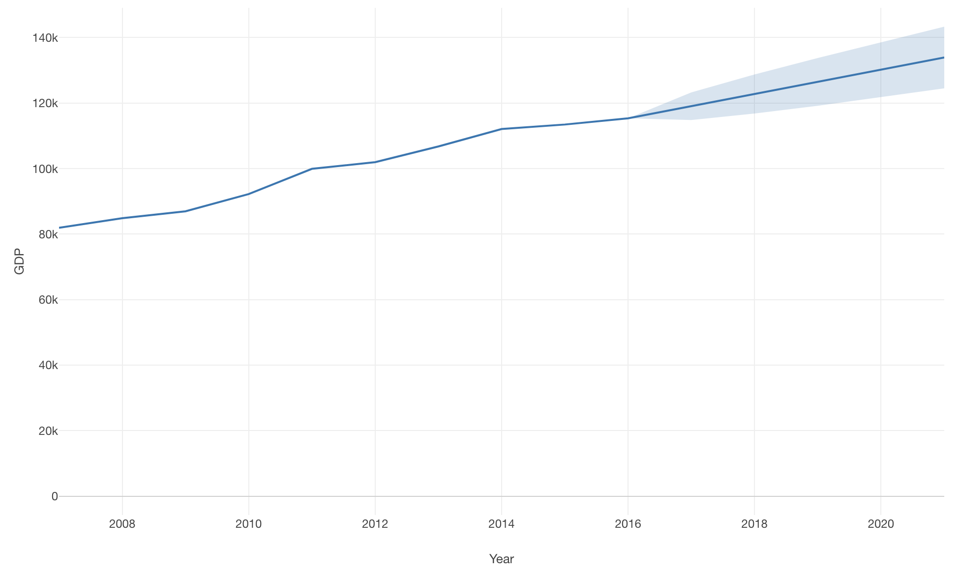
Here is the resulting interactive Line Chart with prediction interval.
If we use only up to 2012 as training data, and compare the forecast with actual data, it looks like this. (As a reference, prediction from prophet is in this chart too.)