Calculating Autocorrelation Function (ACF) for Multiple Time Series

Data

As an example, let's use this data of average flight departure delay (DEP_DELAY) for each day (FL_DATE) for each airline company (CARRIER) in the U.S, which looks like this.

Since there are 16 airlines, there are 16 time series in this data. Let's calculate 16 ACF results for those airlines.

Grouping the Data

Let's group the data by CARRIER, so that the ACF calculation to follow will be done per CARRIER, by adding a Group By step.

Calculate ACF

Now we can calculate ACF by using acf function that comes with base R. Create a Custom R Command step with the following script.

do(ACF=acf(.$DEP_DELAY, plot=FALSE))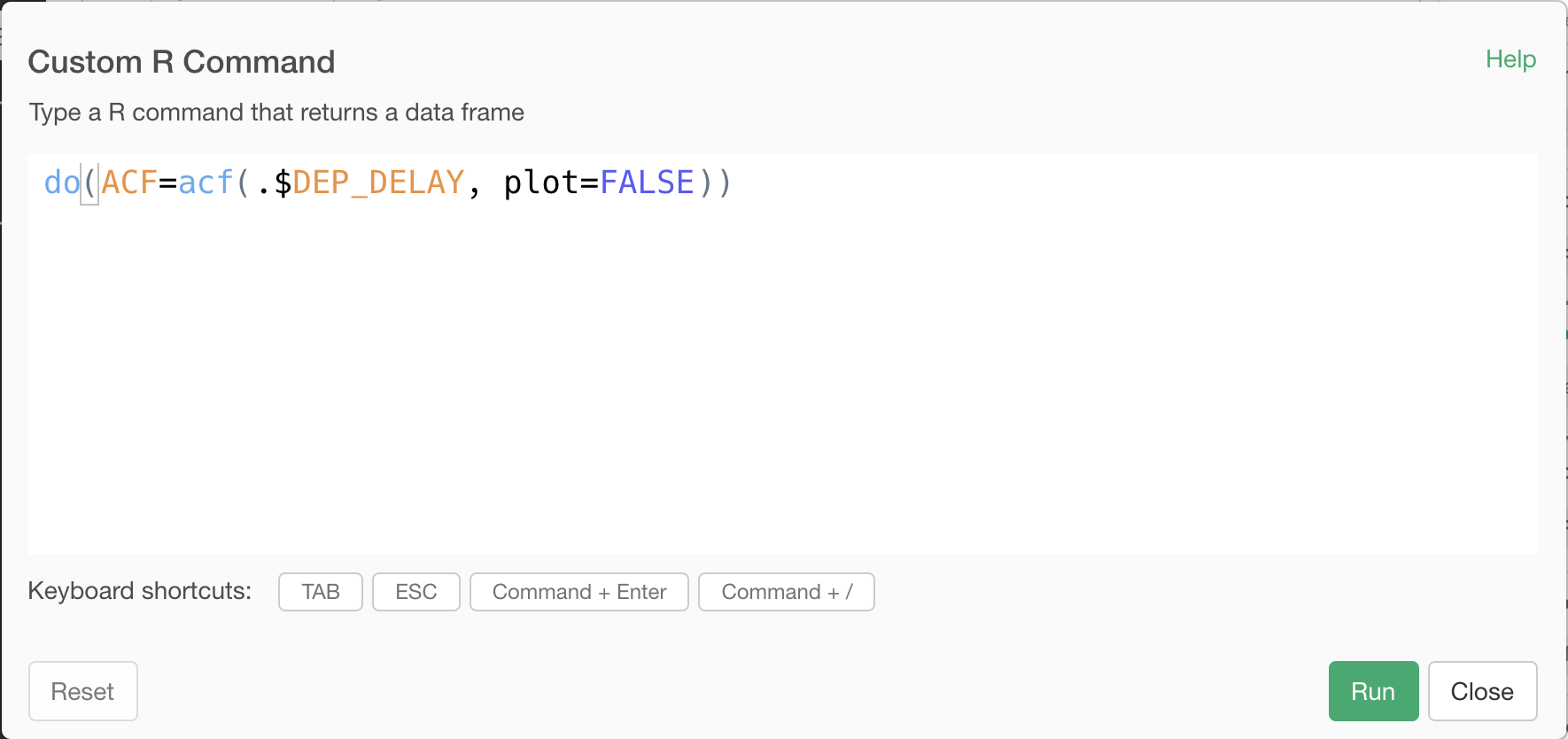

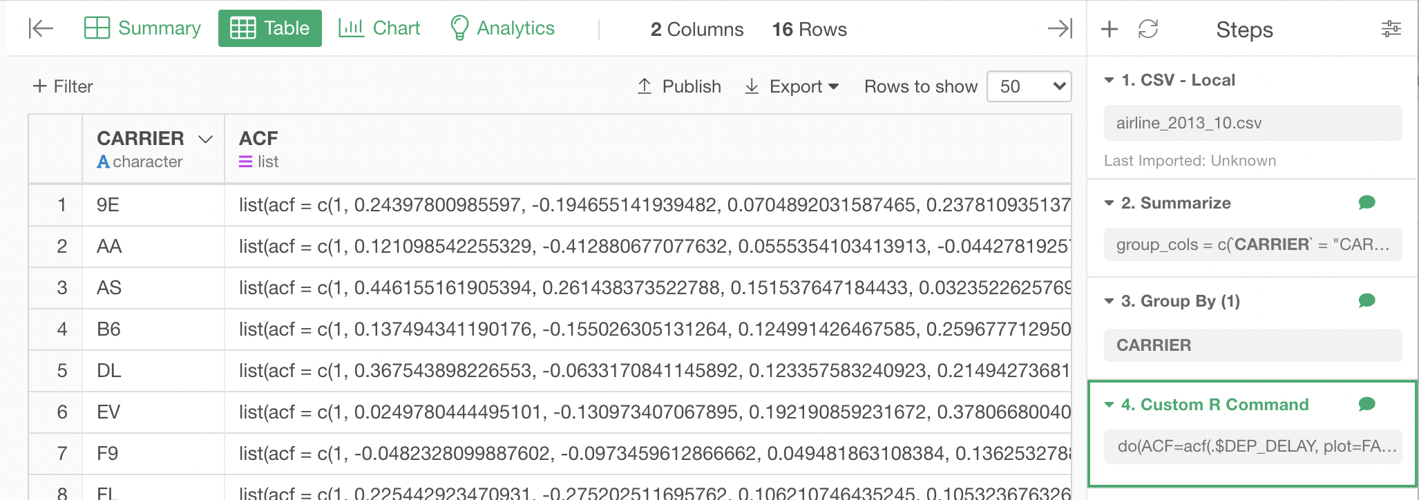
The result of this step looks like the following. The ACF column is a list of ACF object. To extract the results from these ACF objects in a readable format, we need one more step.

Extract Results from ACF Object List Column

Before extracting the results, just to keep the CARRIER column in the results data frame, let's group the data with CARRIER again.

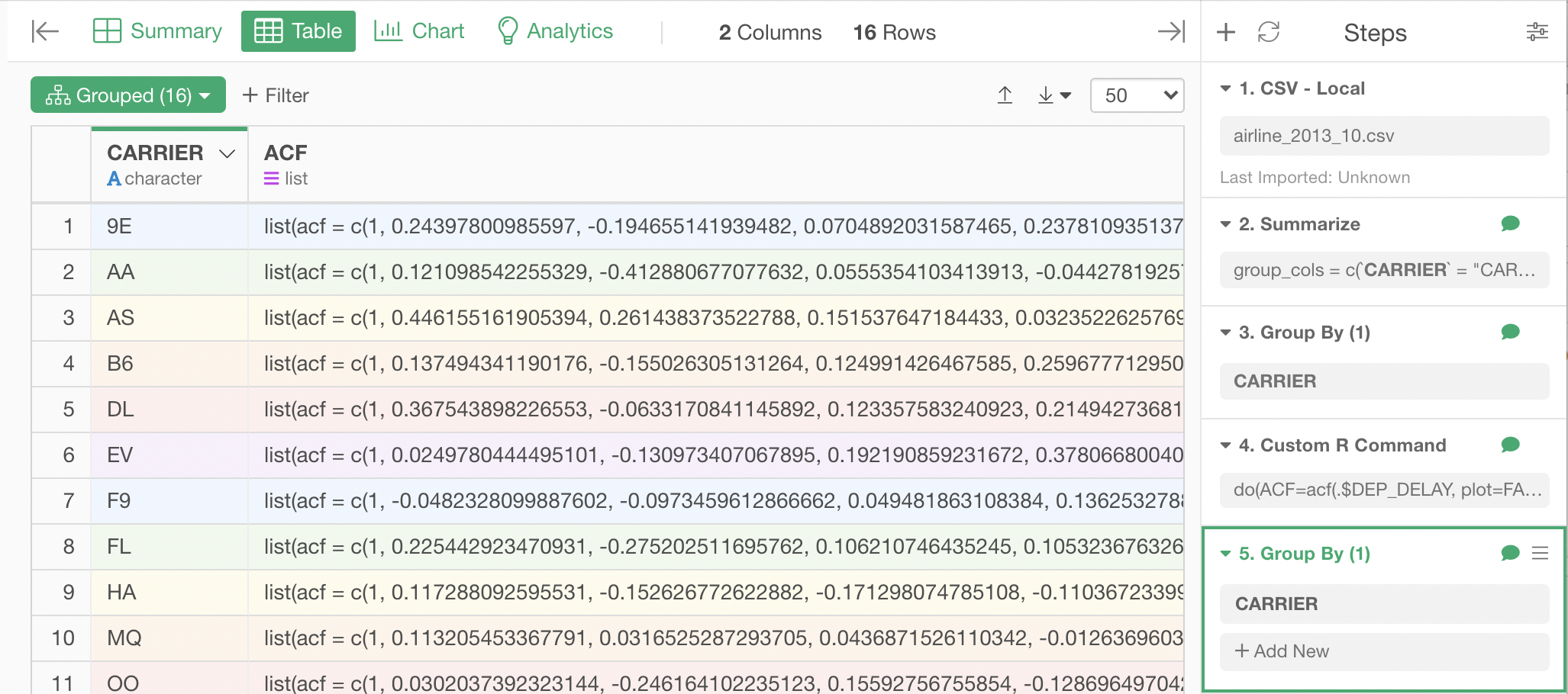
Then, create another Custom R Command step with the following script.

model_info(ACF,output="variables")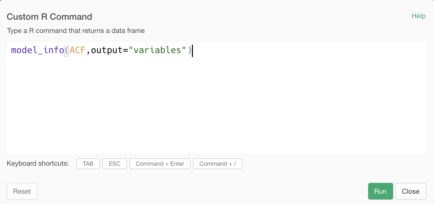

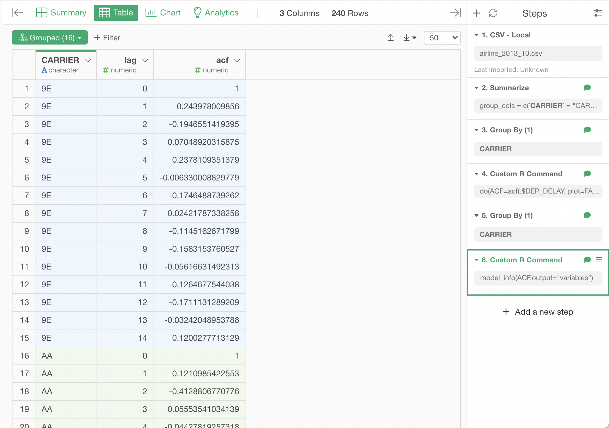
The results look like the following, with ACF values for each lag, for each CARRIER.

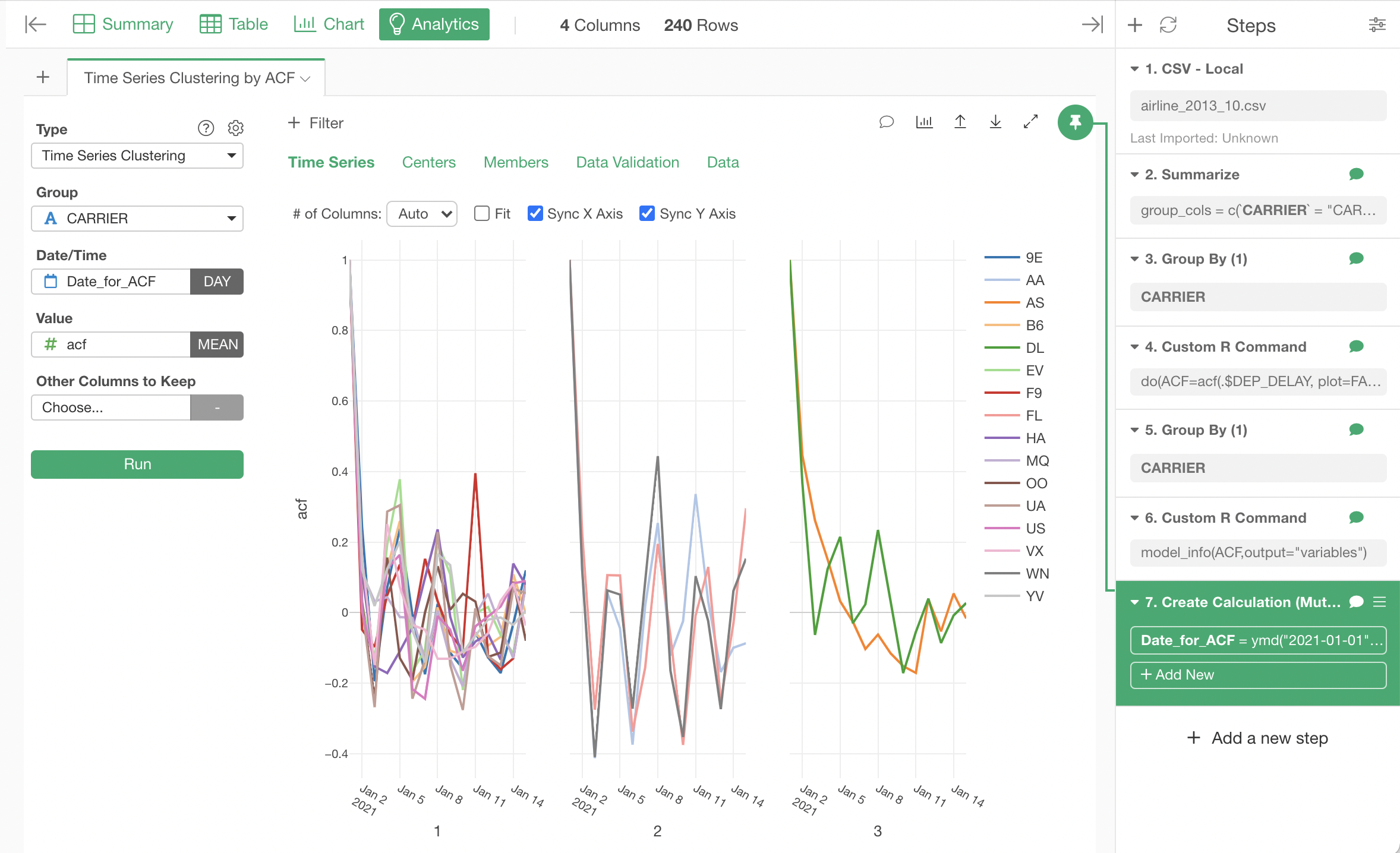
As an example of analysis based on such set of ACF for multiple time series, here is the result of Time Series Clustering based on the above ACF data. It is clustering the airlines based on the view point of what kind of auto correlation their departure delays have as time series.