Calculating Customer Lifetime Value (CLV)

For SaaS (Software-as-a-Service) and subscription businesses, understanding CLV (Customer Lifetime Value) is extremely important.

Unlike one-time purchase businesses, in subscription businesses, the cumulative revenue from the same customer increases over time.

For example, consider a service like Netflix that charges $20 per month.

In the first month, you can only earn $20 in revenue from a customer, but if this customer doesn’t cancel the service for the next 12 months, you can earn a total of $240 from this customer.

This is called Customer Lifetime Value or CLV.

Understanding how much revenue can be expected from one customer is important because it helps determine how much can be spent on acquiring new customers and retaining existing ones.

CLV can be calculated using the following three methods, which will be introduced in this Note:

Estimating CLV by intuition
Estimating CLV from churn rate
Estimating CLV from survival rate

Estimating CLV by Intuition

Let’s start with the simplest method.

For example, if you assume the average customer duration is about 12 months, and the monthly revenue per customer is $100, the CLV becomes $1,200.

12 * 100 = 1200

However, this calculation might be too simplistic. This is because the 12-month figure has no basis, and it assumes that no one churns when estimating CLV.

Unfortunately, customers churn in any business, so such an estimate is not realistic.

Estimating CLV from Churn Rate

The average customer duration is greatly influenced by the churn rate. For example, if the customer churn rate is high, the average duration will be short, and if the churn rate is low, the average duration will be long.

The average customer duration can be calculated as follows:

Average Lifetime = 1 / Churn Rate

For example, if the monthly churn rate is 10%, the average duration can be calculated as follows:

1 / 0.1 = 10

The average duration is 10 months as shown above.

After calculating the average duration, CLV can be calculated by multiplying it by the monthly revenue per customer.

If the monthly revenue per customer is $100, the CLV becomes $1,000.

10 * 100 = 1,000

However, there is a problem with this calculation.

Since churn rates vary by month, you cannot expect the same monthly revenue every month.

For example, the churn rate might be 40% in the first month, 30% in the second month, and then flatten out at 25% thereafter.

Therefore, if you want to calculate CLV in a more realistic way, it’s better to calculate the retention rate (survival rate) for each period throughout the customer’s lifetime and multiply these values by the monthly revenue.

Estimating CLV from Survival Rate

The most appropriate way to estimate the survival rate (or retention rate) from the time of customer conversion is to use the Kaplan-Meier method, a well-known statistical algorithm.

The advantage of the Kaplan-Meier method is that it can account for users who have just converted and started using the service recently, as well as users whose churn status is unknown.

In Exploratory, you can calculate and visualize the survival rate from the time of customer conversion using the Kaplan-Meier method from the “Survival Curve” in the Analytics view.

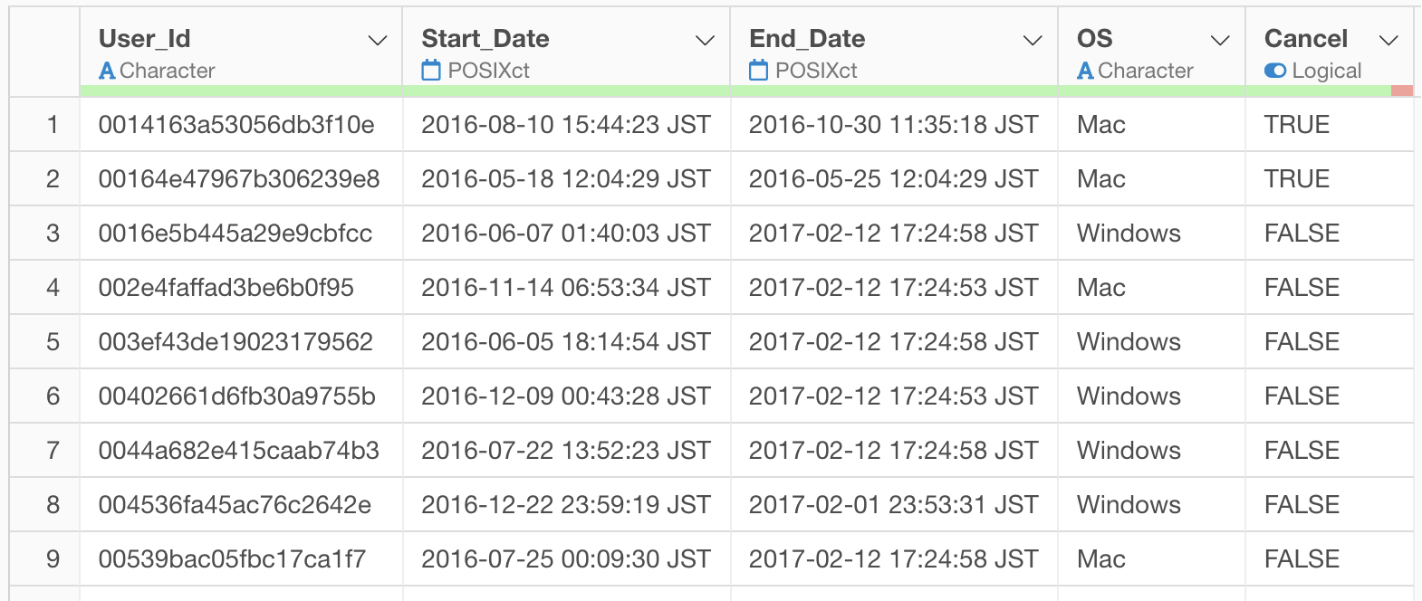
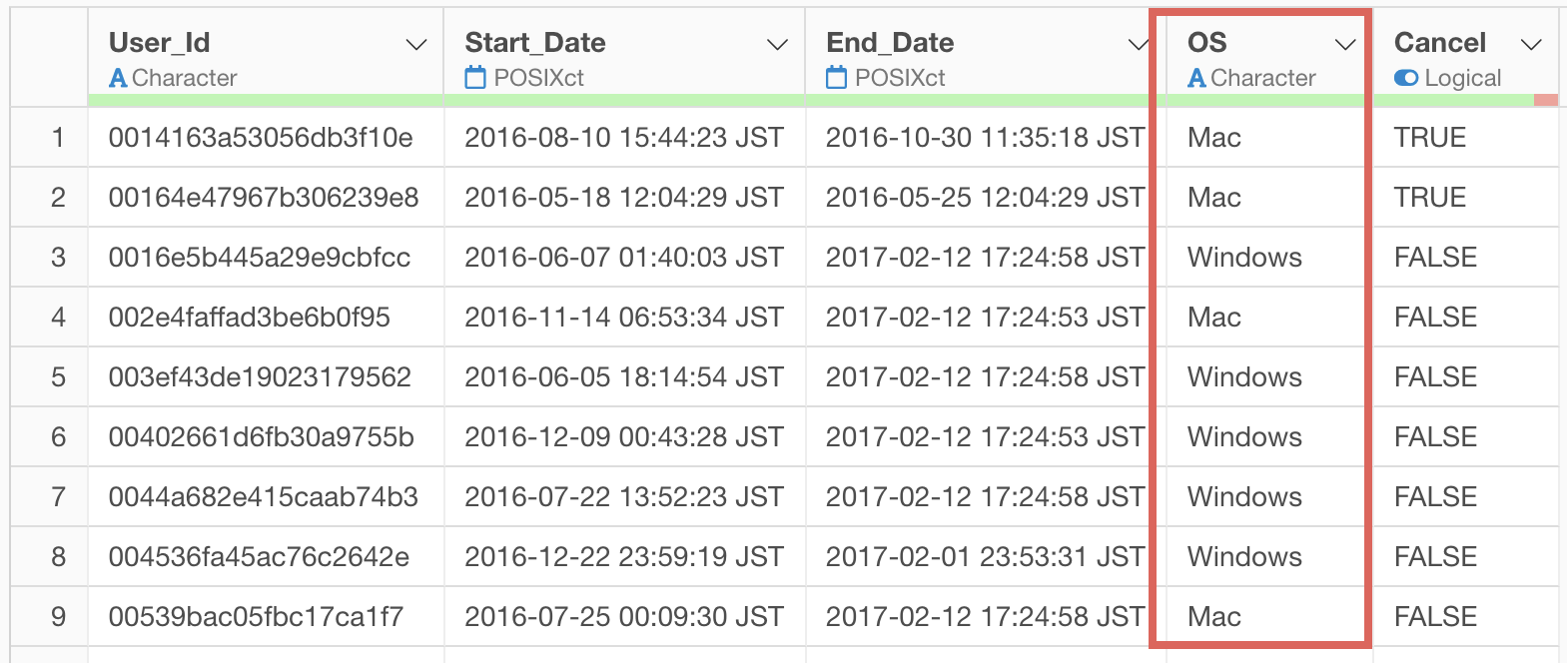
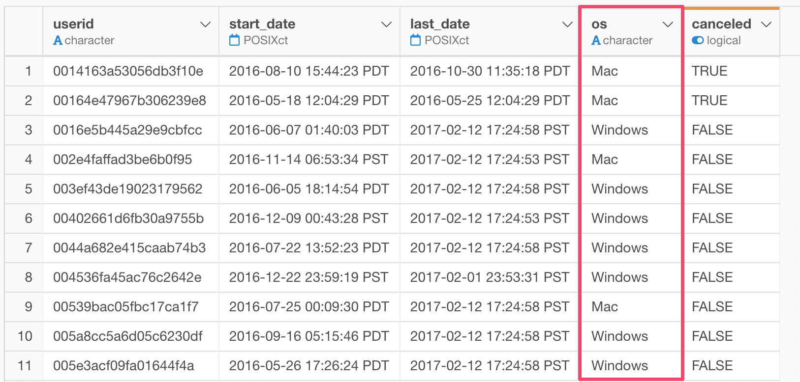
From here, I’ll introduce how to calculate CLV from survival rates using data where each row represents one customer and includes the following information. (You can download the data from here)

User ID
Start Date - The date the customer started using the service
End Date - The date the customer stopped using the service
OS - Information about the operating system being used
Cancel - Whether the service was canceled or not

Take a look at this note on how to prepare the data for Survival Curve.

In Exploratory, there are two methods for creating metrics:

AI Prompt: Creating metrics using a feature that processes data with natural language
UI Menu: Creating metrics by processing data through menus accessible from the UI

This Note will introduce both methods.

“AI Prompt” is only available for users with paid licenses such as Business Plan or Personal Plan, or users who are currently trialing these plans.

Also, AI Prompt is only available when your device is connected to the internet.

If you are not using the above plans, or if you are using a device that is not connected to the internet, please proceed to the “Calculating CLV with UI” section.

Calculating CLV with AI Prompt

This section introduces how to create metrics using AI Prompt. (For details on AI Prompt, please see here.

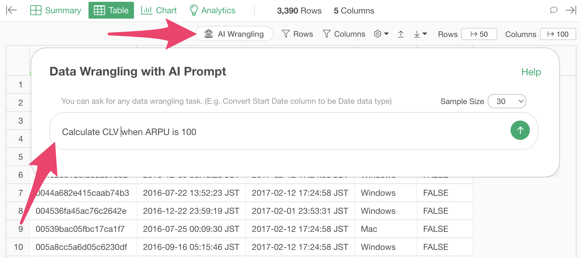
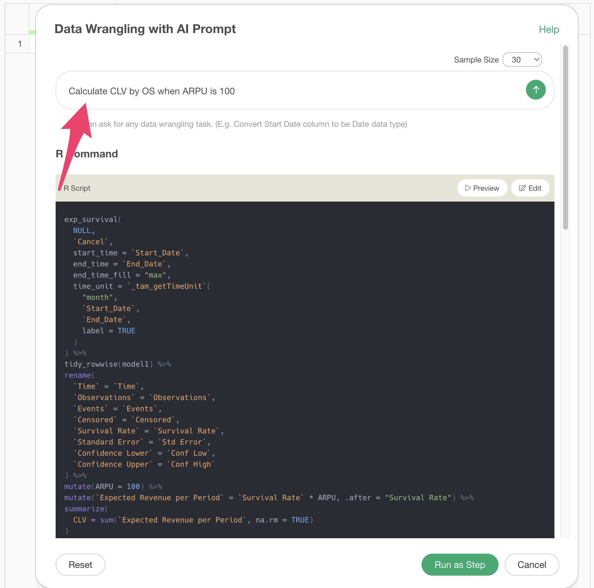
First, click the “AI Wrangling” button, and when the AI Prompt dialog appears, enter text like the following and execute:

Calculate CLV when ARPU is 100

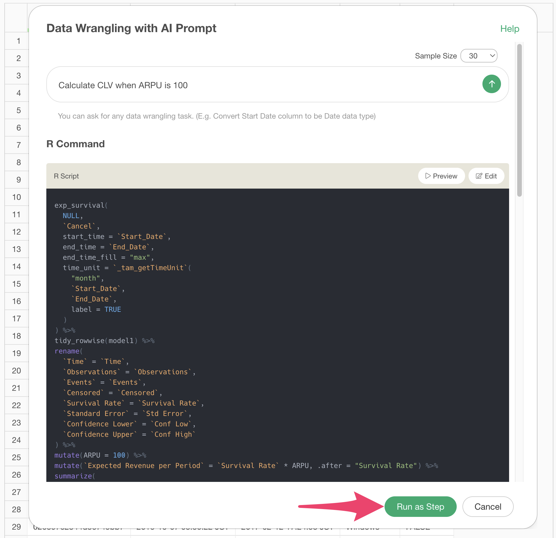
This will generate code to calculate CLV using the survival curve, assuming an ARPU (Average Revenue Per User) of $100. Check the results and click the “Run as Step” button.

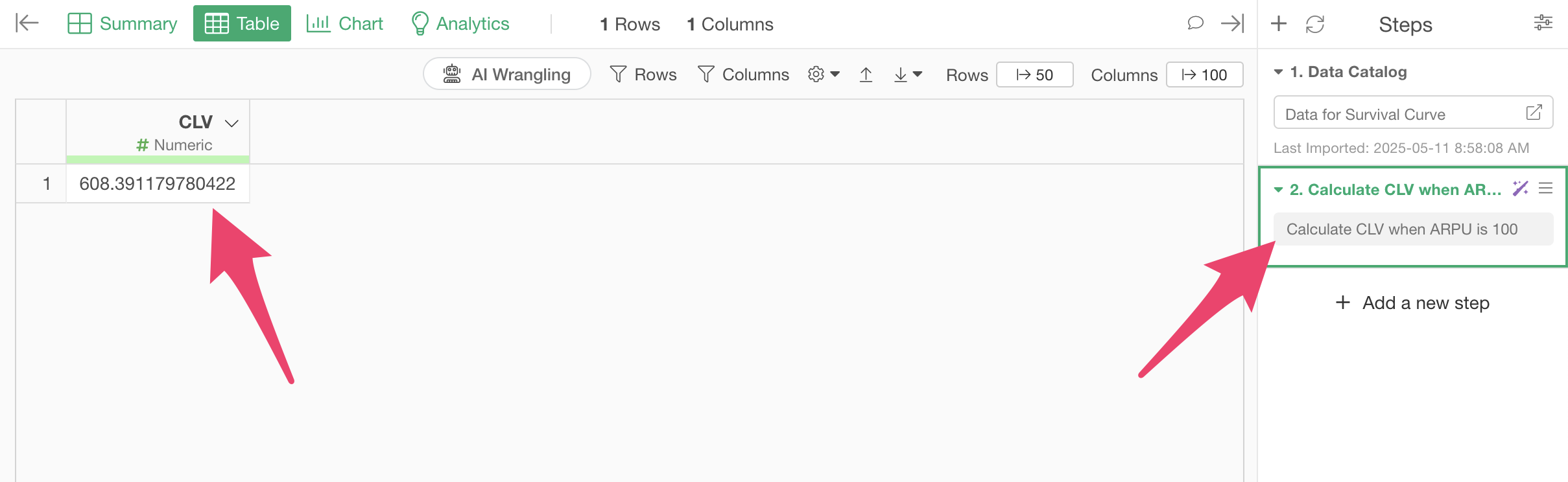
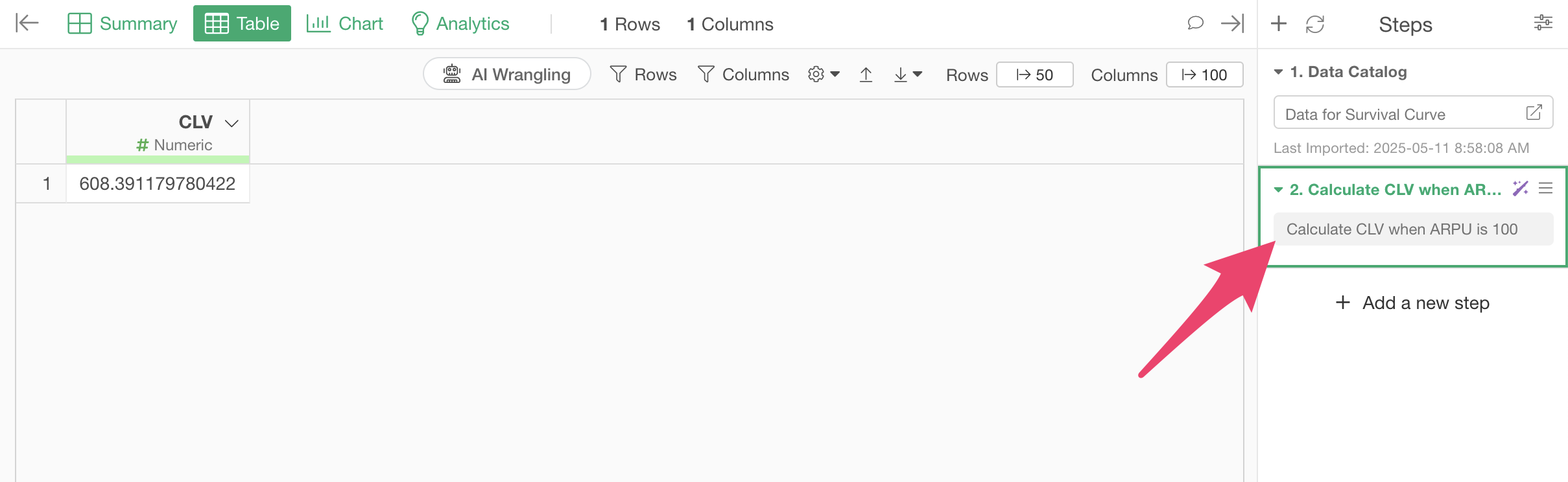
The step is added, and CLV has been calculated.

Calculating CLV by Segment

By the way, the original data had a column showing which PC OS each user was using.

If you want to know if there’s a difference in CLV between Windows and Mac users, and if so, how much, you can easily calculate CLV for each.

Open the step that calculates CLV that was added earlier.

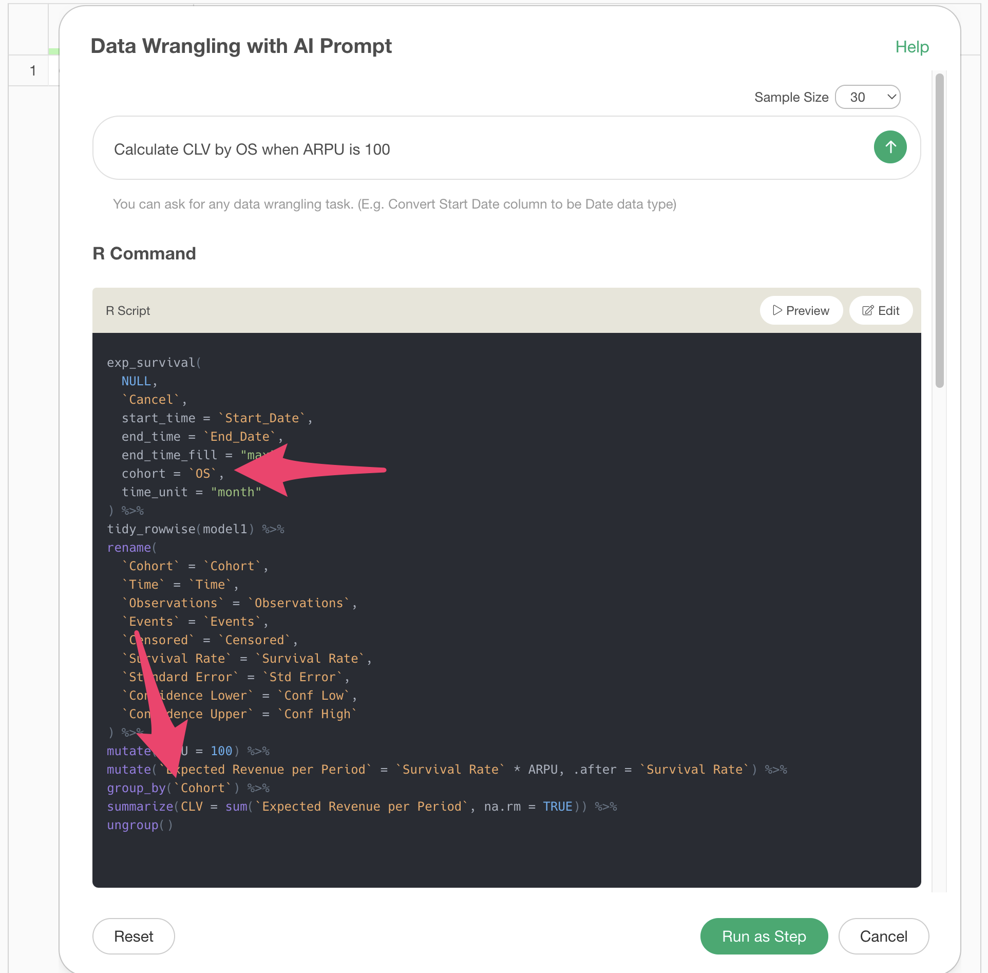
When the AI Prompt dialog opens, change the prompt to text like the following and execute:

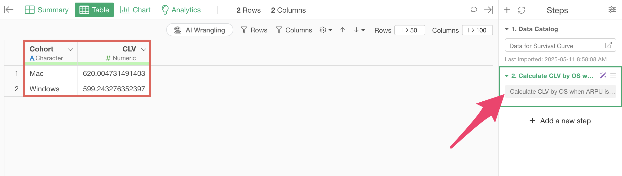
Calculate CLV by OS when ARPU is $100

This will regenerate code to create survival curves by OS and calculate CLV assuming an ARPU of $100. Check the results and click the “Run as Step” button.

Now you’ve calculated CLV by OS.

Calculating CLV with UI

Finding Survival Rate Using Survival Curve

Go to the Analytics view and select “Survival Curve” as the type.

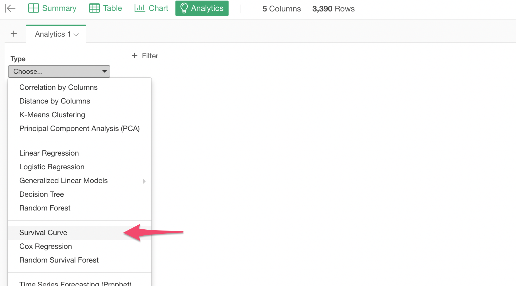
Then select the following columns for each item and execute:

Start Date -> Start Time
End Date -> End Time
Survival Status (Event) -> Cancel

You’ve created a survival curve.

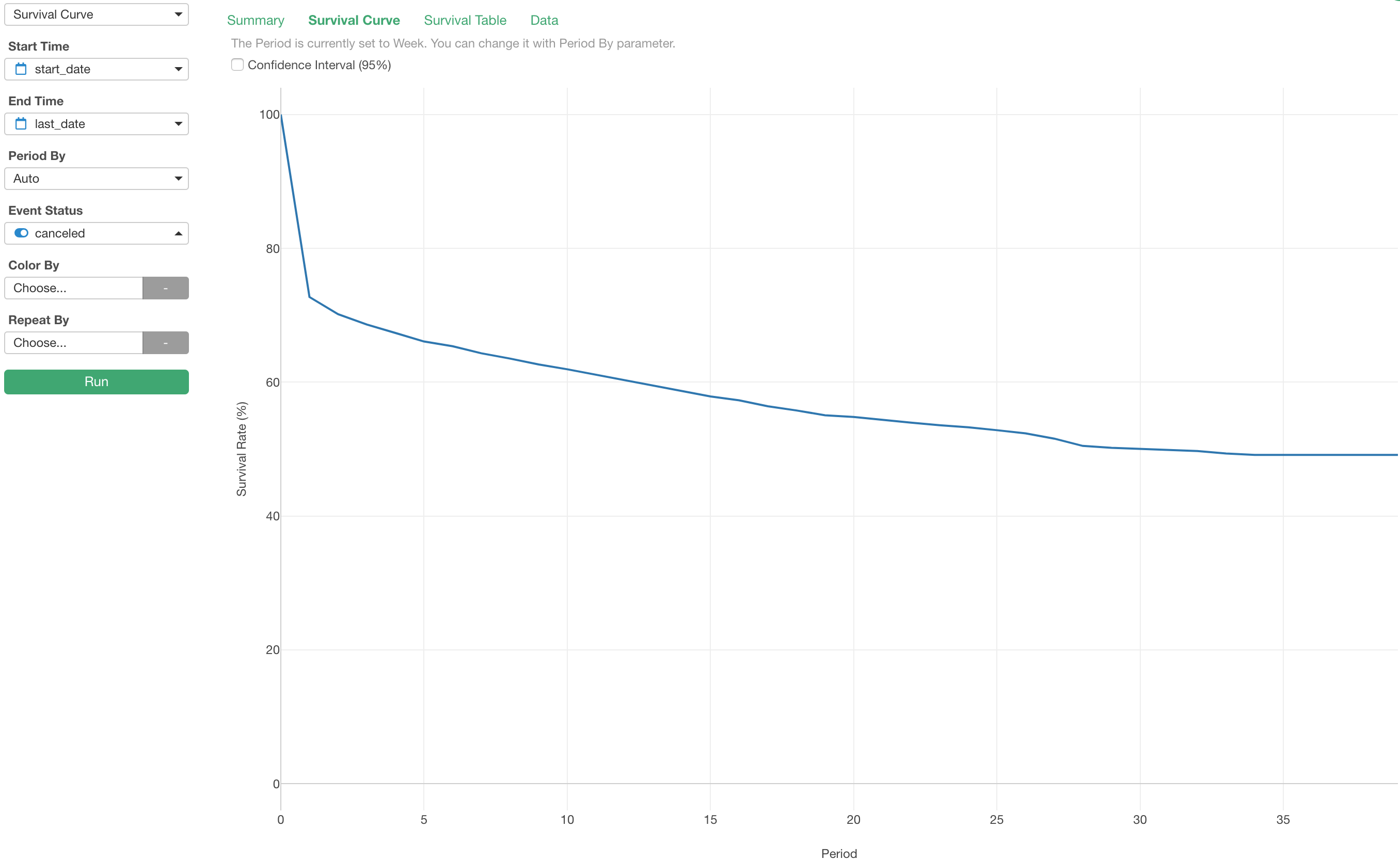
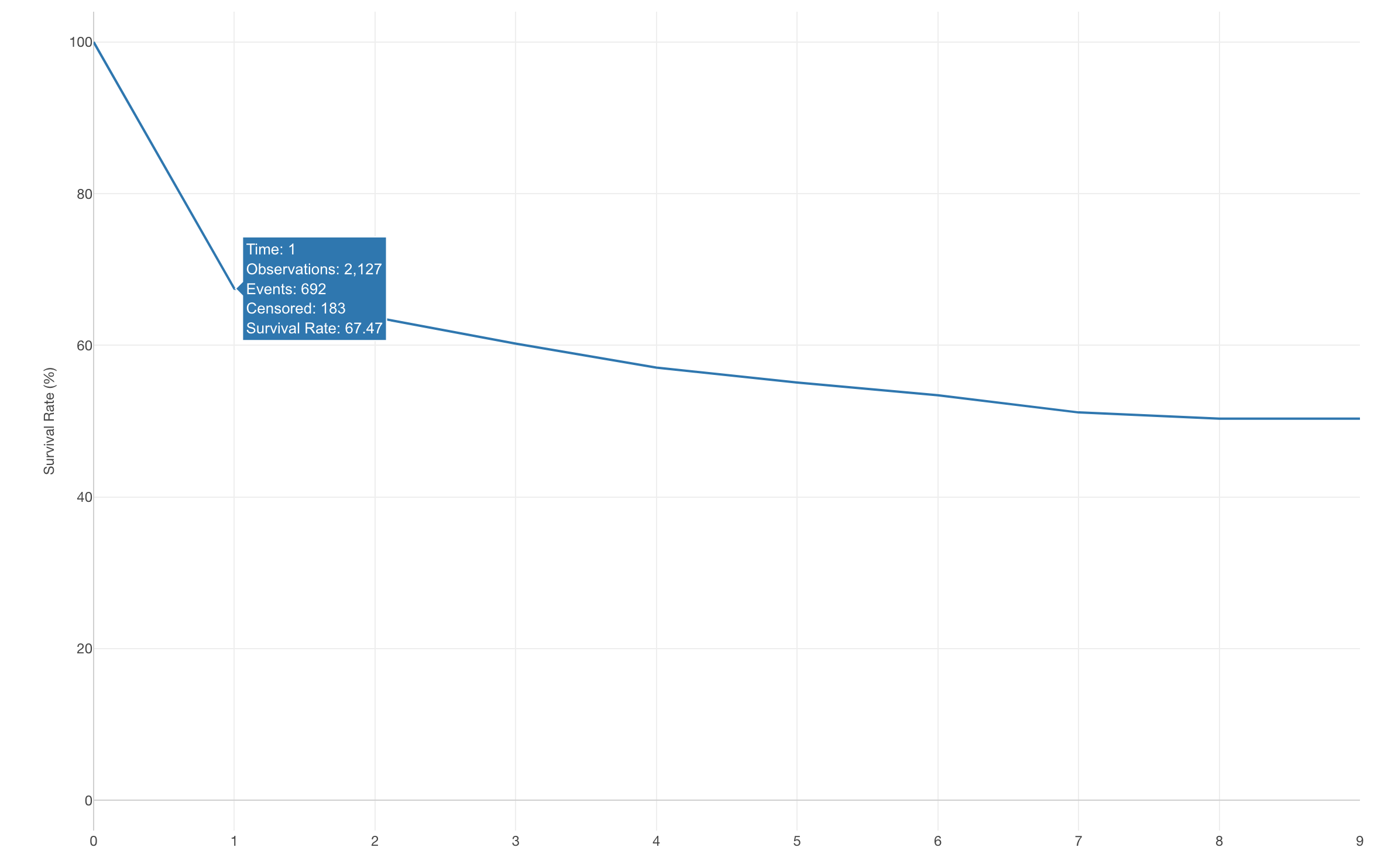
This “Survival Curve” chart shows the survival rate for each period. Currently, the period is set to “week”.

Let’s change the period unit to “month” to visualize the survival rate for each elapsed month.

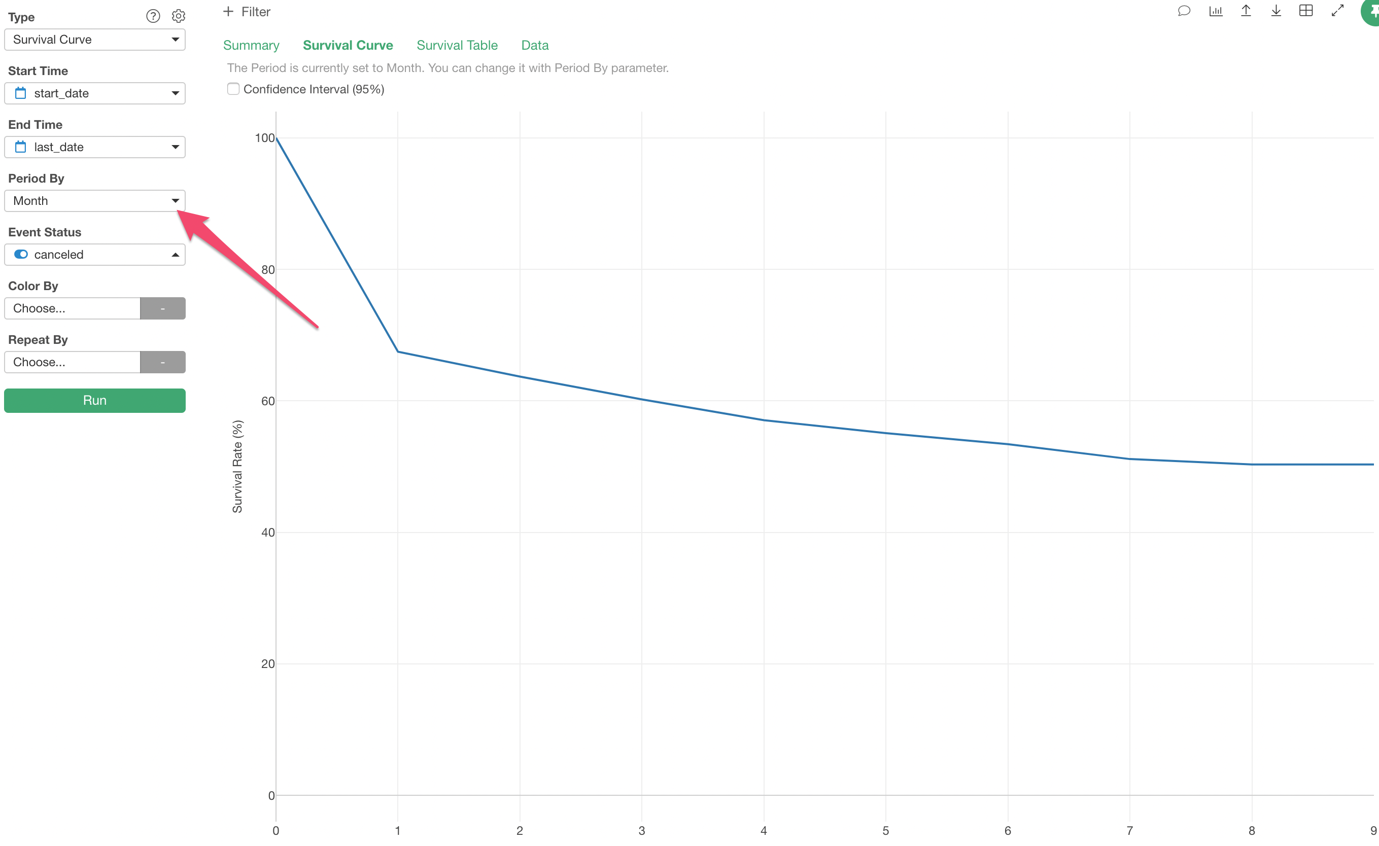
Now you can visualize the survival rate by month.

For example, you can see that the survival rate for the first month is 67.47%.

So how do we use this survival curve to calculate CLV (Customer Lifetime Value)?

To reiterate, CLV is the expected revenue from a customer from the time they convert until they churn.

Therefore, the expected revenue for each period can be calculated as follows:

Expected Revenue of a given period = Survival Rate of the period * Recurring Revenue

Looking at the survival curve, the period where the X-axis is 0 represents the time of conversion, so it starts at 100%.

If the monthly fee for this service is $100, then $100 in revenue can be expected per customer.

The survival rate for the second month is 67.47%.

What this tells us is that the expected revenue per customer for this period is not $100, but about $67.

If this explanation doesn’t raise any questions, you can skip it and move on to the next section. If you have questions about this explanation, please continue reading.

If there were initially 100 customers, a survival rate of 67% means that only 67 customers remain by the end of this period.

This means that revenue can only be expected from these 67 customers. Since the monthly fee for this service is $100, the total revenue is $6,700.

67 * $100 (revenue per person) = $6700

Since there were originally 100 customers, to calculate the average revenue per customer, divide $6,700 by 100 to get $67, which means you’re doing the following calculation:

0.67 (67%) * $100 (recurring revenue per person) = $67

In this way, you can calculate the expected revenue for each period by multiplying the monthly revenue per person by the survival rate for that period.

The third month is similar.

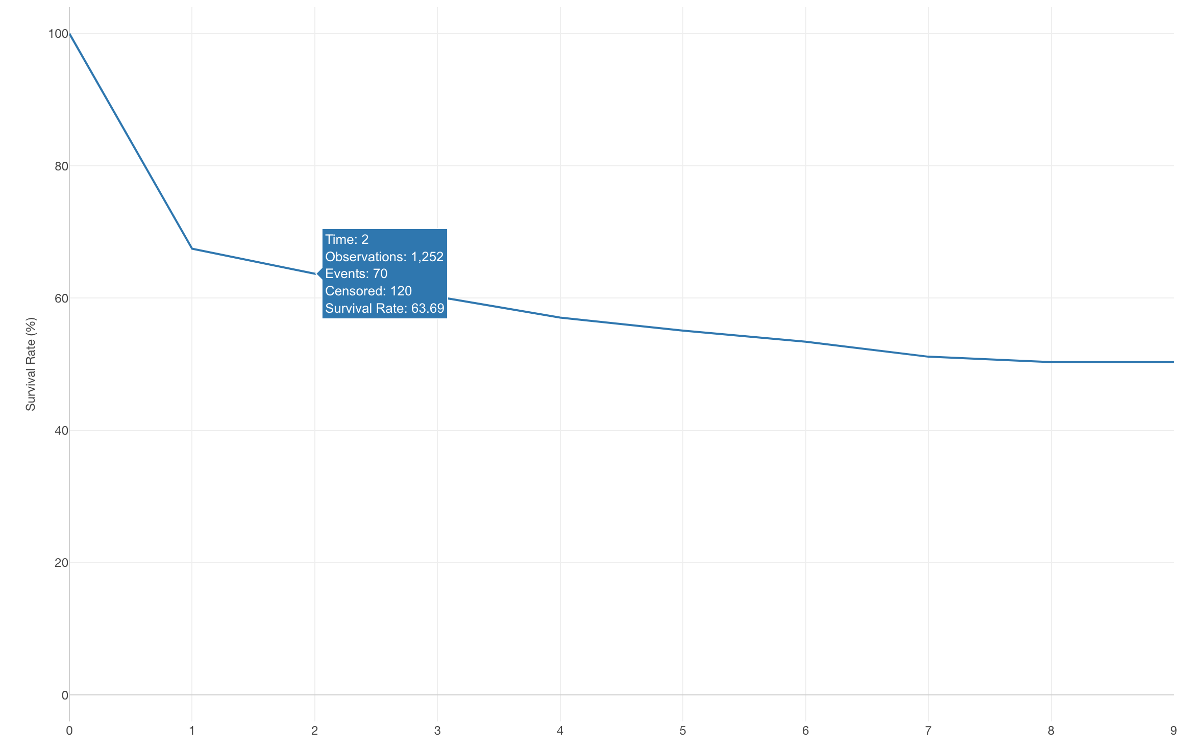
The survival rate is about 63%, so the expected revenue per customer for this period is $63.

0.63 * $100 = $63

Like expected revenue, survival rates tend to decrease over time, and CLV is the sum of the expected revenue for all periods until everyone churns.

Now that we understand the logic of calculating CLV using survival rates, let’s actually calculate it in Exploratory.

Calculating CLV Using Survival Rate

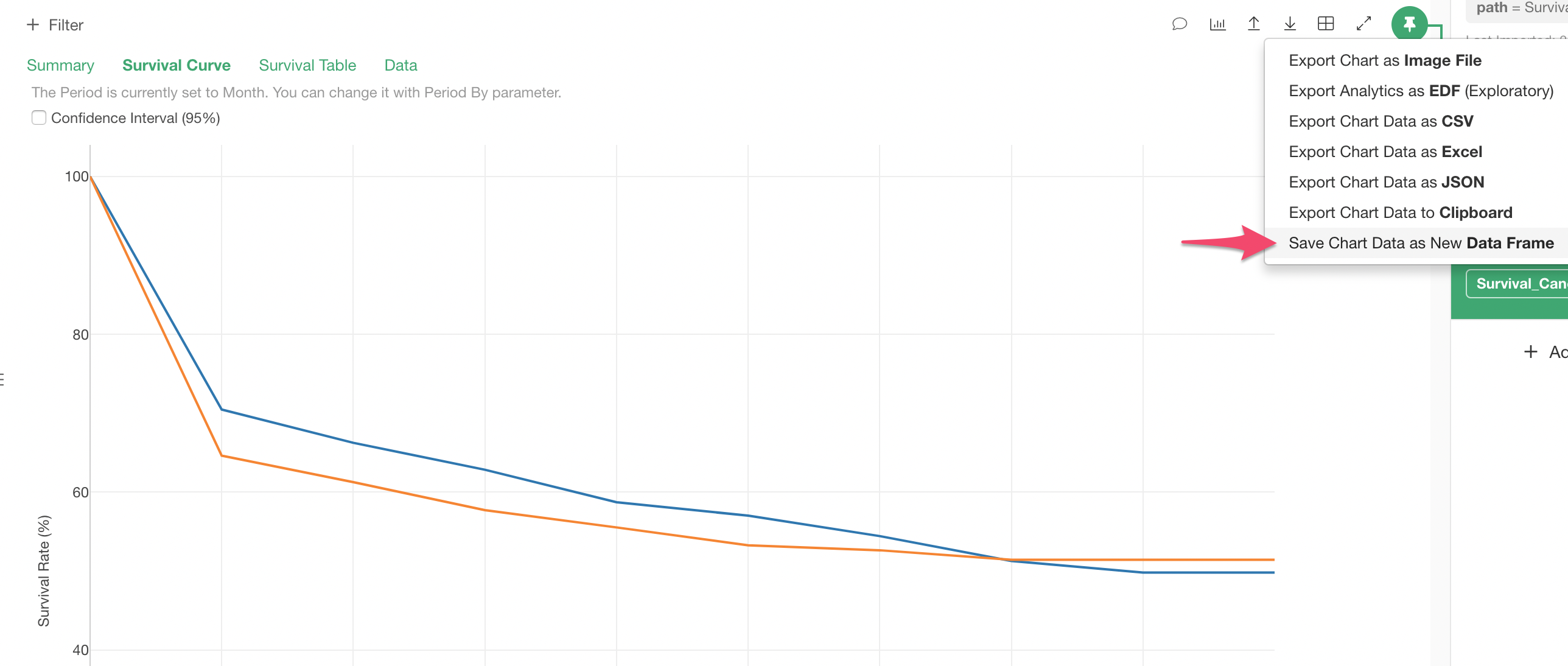
Click the “Export” button and select “Save Chart Data as New Data Frame”.

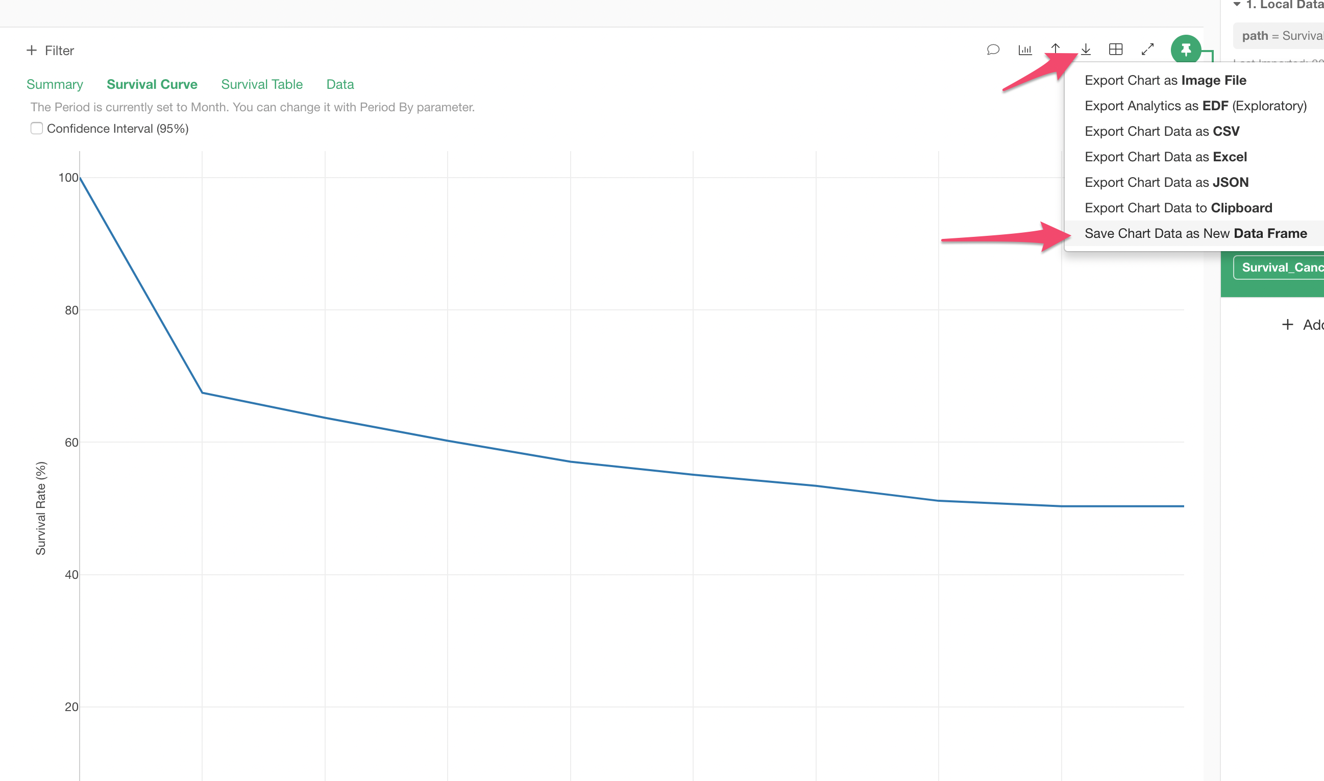
This creates a new data frame based on the exported data.

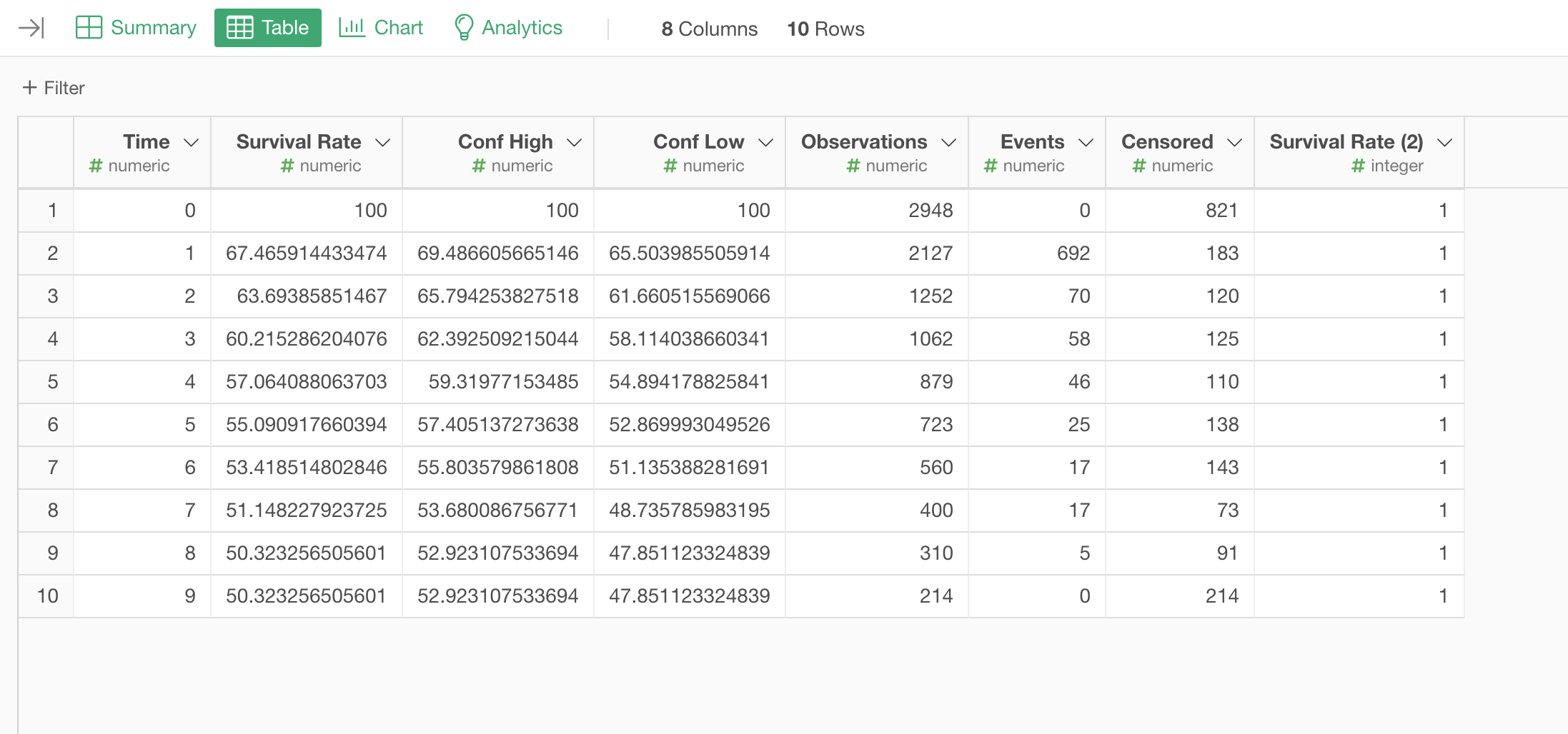
Now you can calculate CLV.

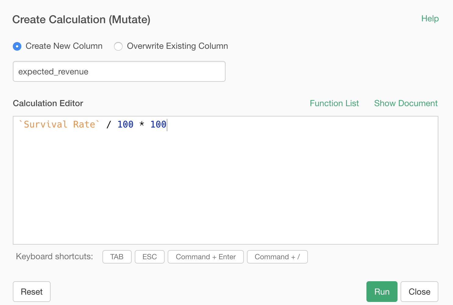
From the “Survival Rate” column header menu, select “Create Calculation (Mutate)”.

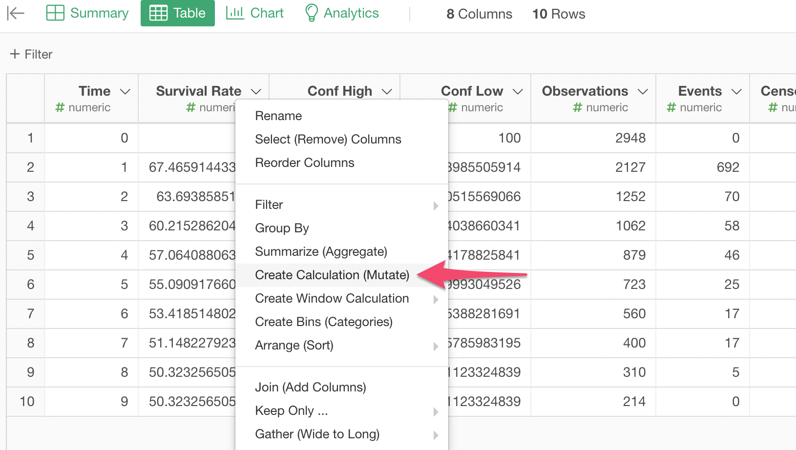
Since the “Survival Rate” column is a column with percentage as the unit, you need to divide it by 100 and then multiply it by the monthly revenue of $100.

Enter the following formula and execute:

`Survival Rate`/ 100 * 100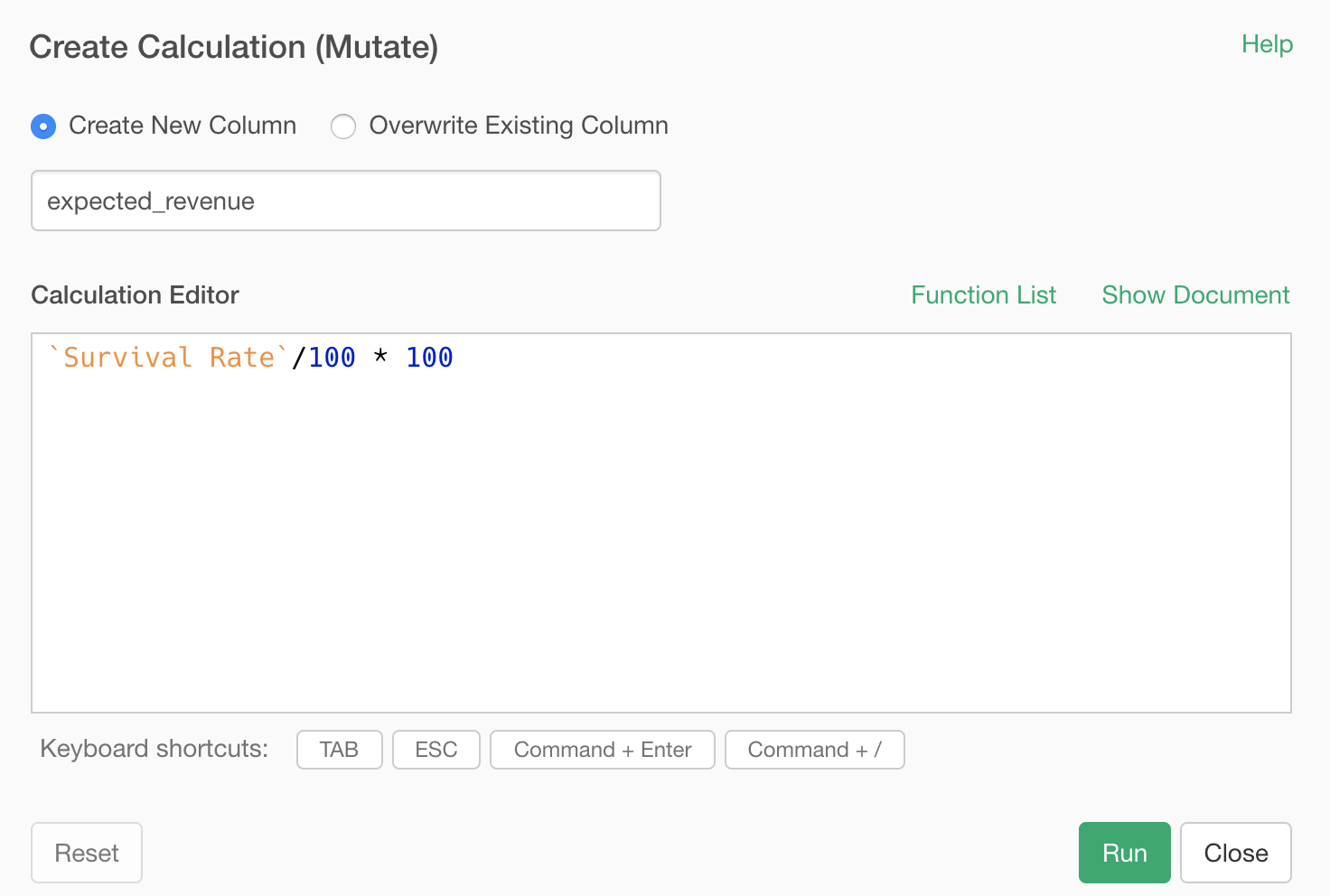

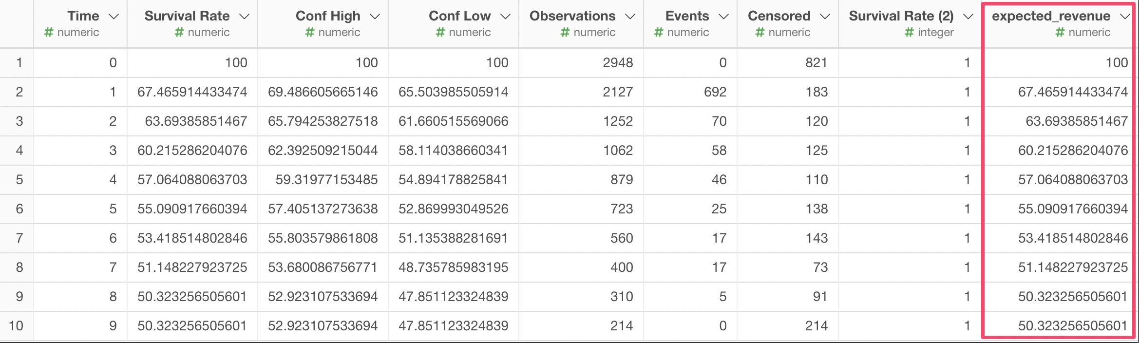
Now that you’ve calculated the expected revenue for all periods, all that’s left is to sum up these revenues.

The easiest way is to aggregate using a pivot table from the Chart view.

Select the expected revenue column for the value and select SUM as the aggregation function.

You’ve found that the CLV is $608.74.

Calculating CLV by Segment

Remember that the original data had a column showing which PC OS each user was using?

What if you want to know if there’s a difference in CLV between Windows and Mac users, and if so, how much?

These CLVs can also be easily calculated.

First, create survival curves for each segment.

Go back to the original survival curve created in the Analytics view, assign the “OS” column to the color division, and execute.

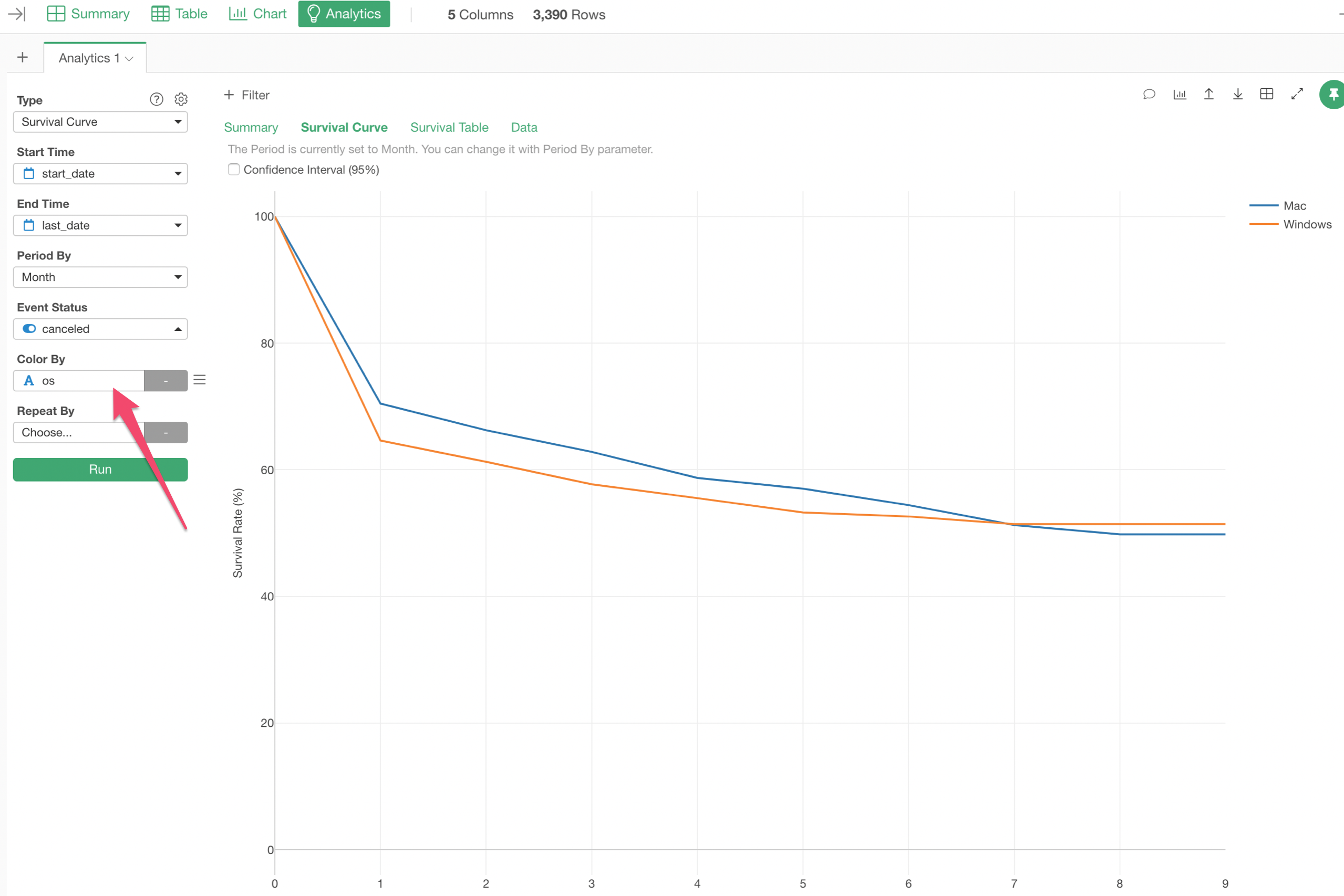
Now you’ve drawn survival curves for Windows and Mac.

Export this data as before and create a new data frame again.

Now you’re ready with data for Mac and Windows.

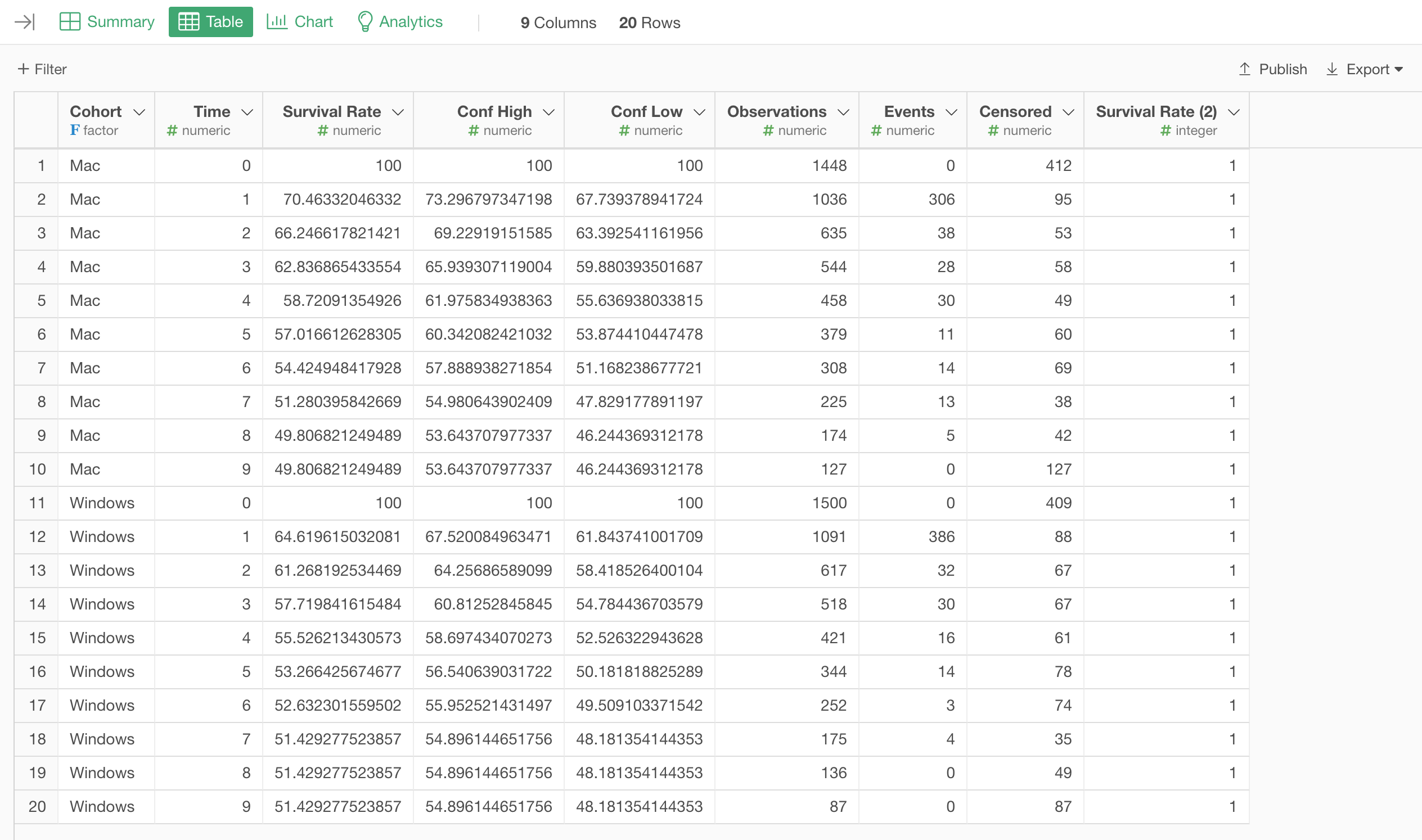
Calculate the expected revenue as before.

Move to the Table view and create a pivot table.

Create a pivot table using the same method as before, but this time assign the “Cohort” column to the rows.

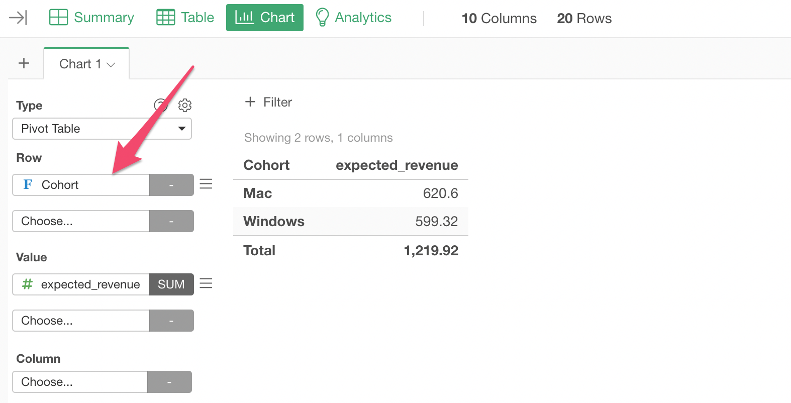
Now you’ve calculated CLV by OS.

The CLV for Mac users is $620.60, and the CLV for Windows users is $599.37.

Points to Consider

Calculating CLV using survival rates is a superior method compared to simply multiplying the same monthly revenue for all periods, as it reflects the actual patterns of customer retention (or churn).

On the other hand, there are cases where you might want to consider the following.

When There Is Not Enough Data

In survival curves, survival rates are calculated only for periods where data exists. If only a short time (e.g., 6 months) has passed since the service was launched, the calculated CLV will be the sum of the expected revenue per customer for 6 months, but in many cases, customers might use your service for more than 6 months. (And you would hope so!)

In such cases, you might want to calculate CLV using the simple method introduced earlier, understanding that the reliability of the CLV obtained may not be high (because churn rates change quickly).

Discount Rate

Another consideration is that the value of money can change over time. If interest rates don’t go negative, by depositing $100 in a bank, you can expect more than $100 in value after 3 years. In that sense, $100 today is not the same as $100 three years from now.

This is called the discount rate, and you can calculate CLV more rigorously using the discount rate, but I’ll explain that method in another Note.