How to Calculate Unit Economics

Here, I will introduce how to calculate Unit Economics using actual data.

We will calculate Unit Economics using two datasets.

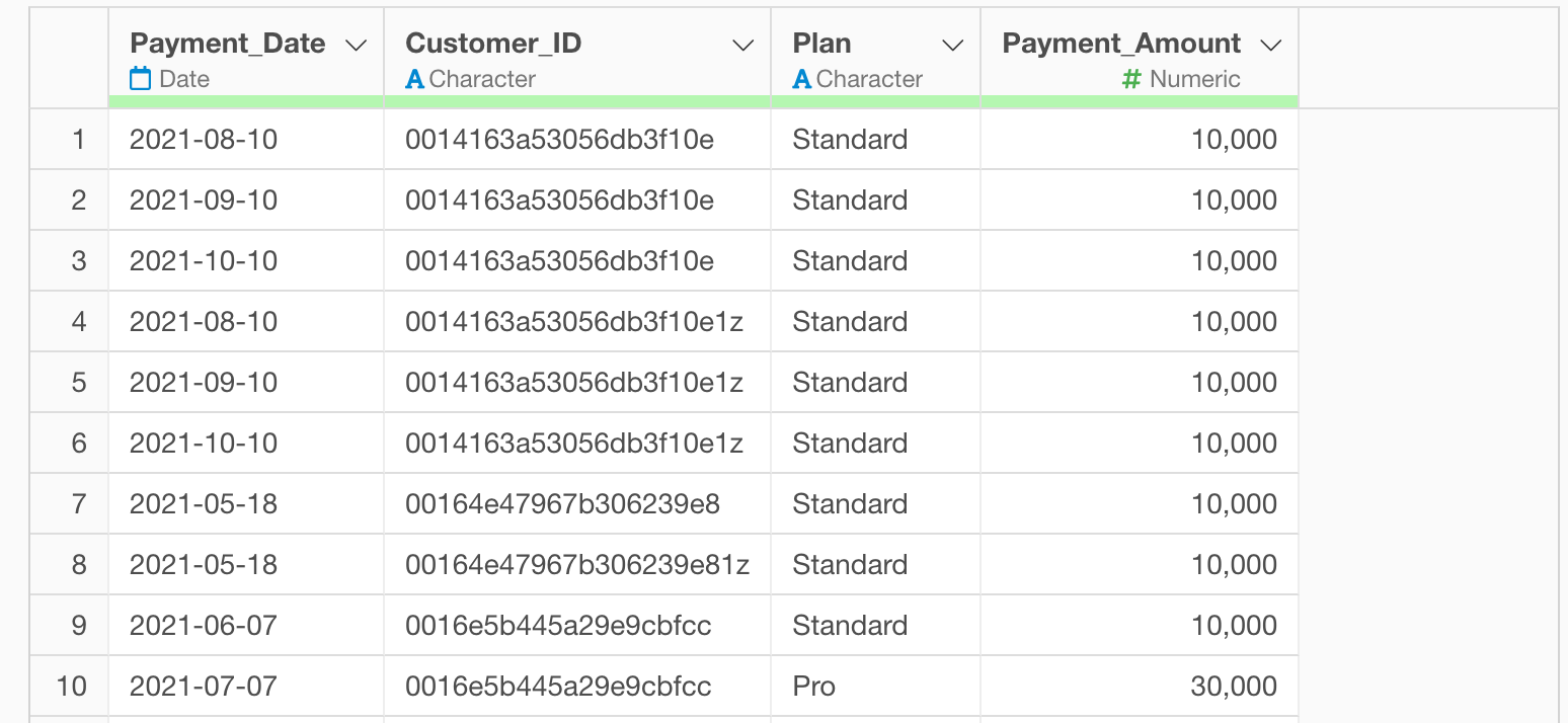
The first dataset represents payment information where each row is one payment transaction, including Customer_ID, Payment_Date, Payment _Amount, and other information. (You can download the data from this page)

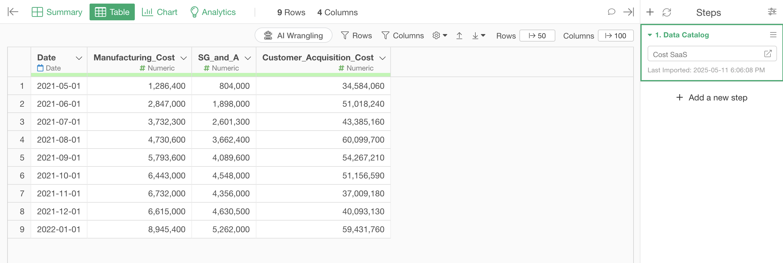
The second dataset contains business cost information where each row represents costs for a particular month. The columns include manufacturing costs, selling and administrative expenses, and acquisition costs for new customers. (The data can be downloaded from this page)

In Exploratory, there are two methods for creating metrics:

AI Prompt: Creating metrics using natural language processing functionality
UI Menu: Creating metrics by processing data through menus accessible from the UI

This note introduces both methods.

“AI Prompt” is only available for users with paid licenses such as Business Plan or Personal Plan, or users who are currently trialing these plans.

Additionally, AI Prompt is only available when your device is connected to the internet.

If you are not using the above plans or are using a device not connected to the internet, please proceed to the “Calculate Unit Economics with UI” section.

Calculate Unit Economics with AI Prompt

This section introduces how to create metrics using AI Prompt. (For details about AI Prompt, please see here.)

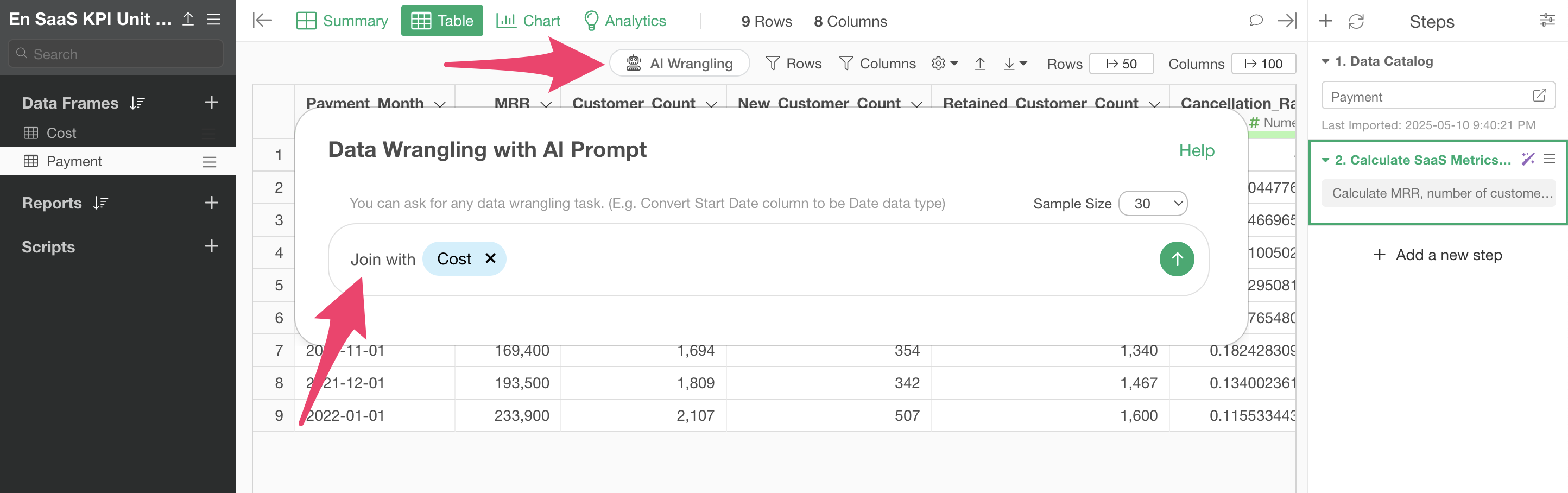
Click the “AI Wrangling” button. When the AI Prompt dialog appears, enter a prompt like the one below and run it:

Calculate MRR, number of customers, number of new customers, number of retained customers, cancellation rate, ARPU, and CLV by month

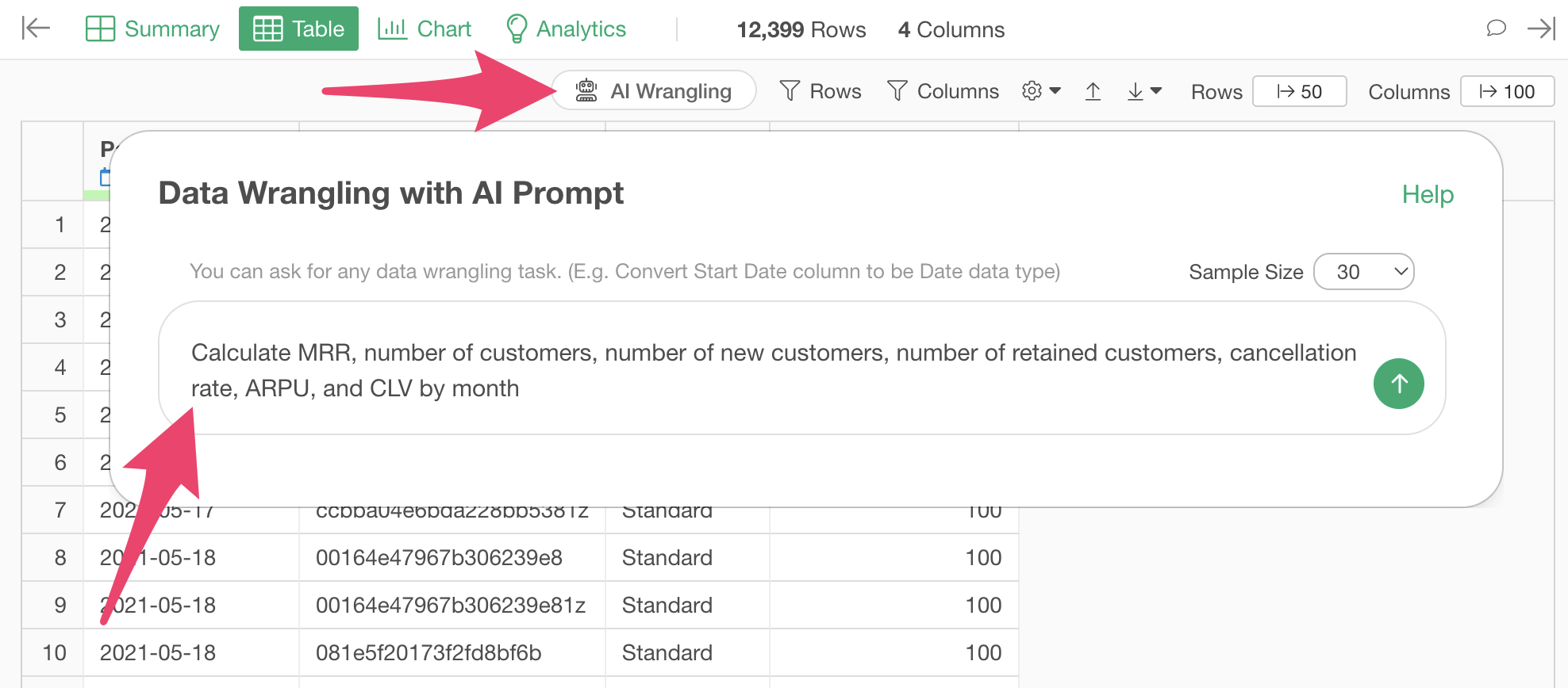
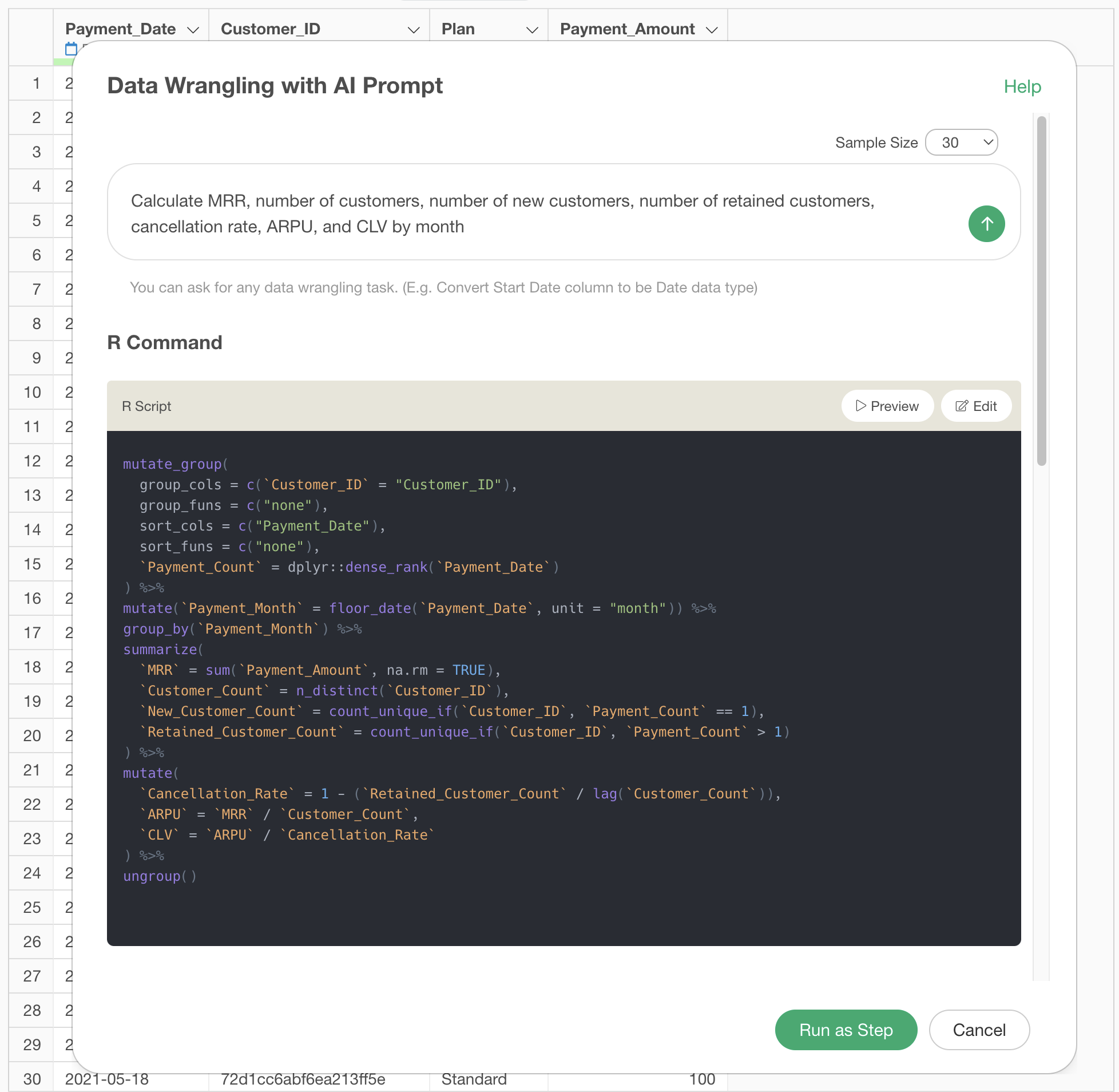
This will generate code to calculate various metrics needed for Unit Economics calculation (MRR, number of customers, number of new customers, number of continuing customers, cancellation rate, ARPU, CLV).

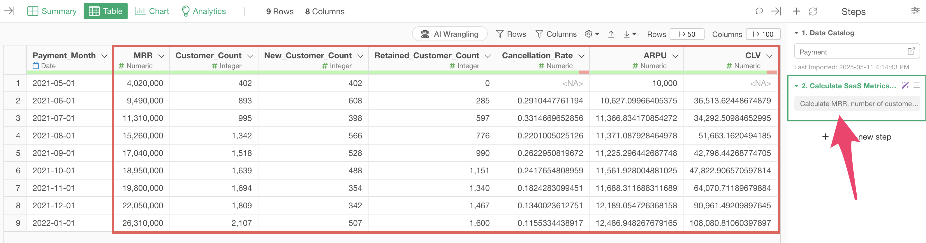
After checking the results, click the “Run as Step” button.

The step is added, and we have calculated monthly basic metrics and customer metrics.

Next, click the “AI Wrangling” button again to join the cost data.

When you want to perform operations that reference other data frames, such as join, you can specify data frames in your project by entering “$”.

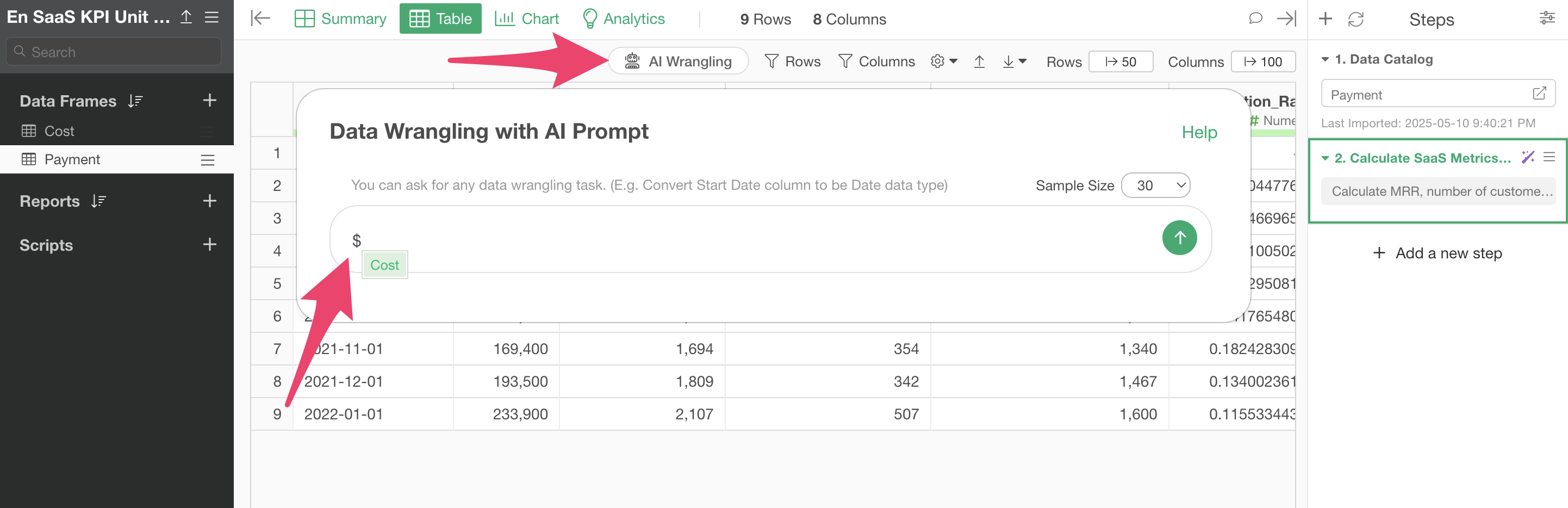
Since we want to join with the cost data, enter text like the following and execute:

Join with cost data

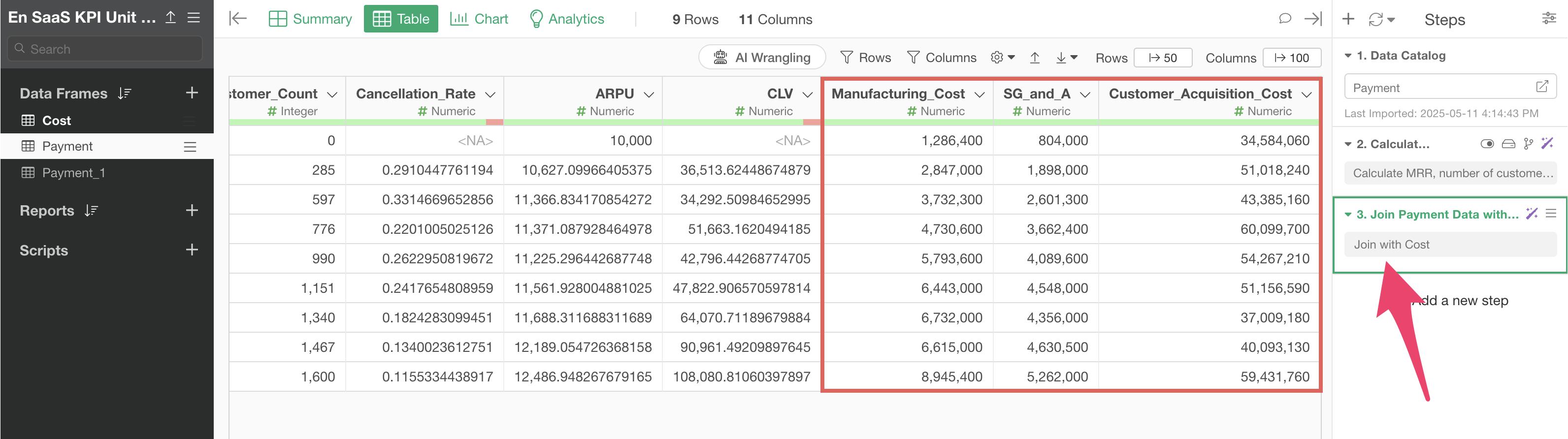
This will generate code to join the cost data. After checking the results, click the “Run as Step” button.

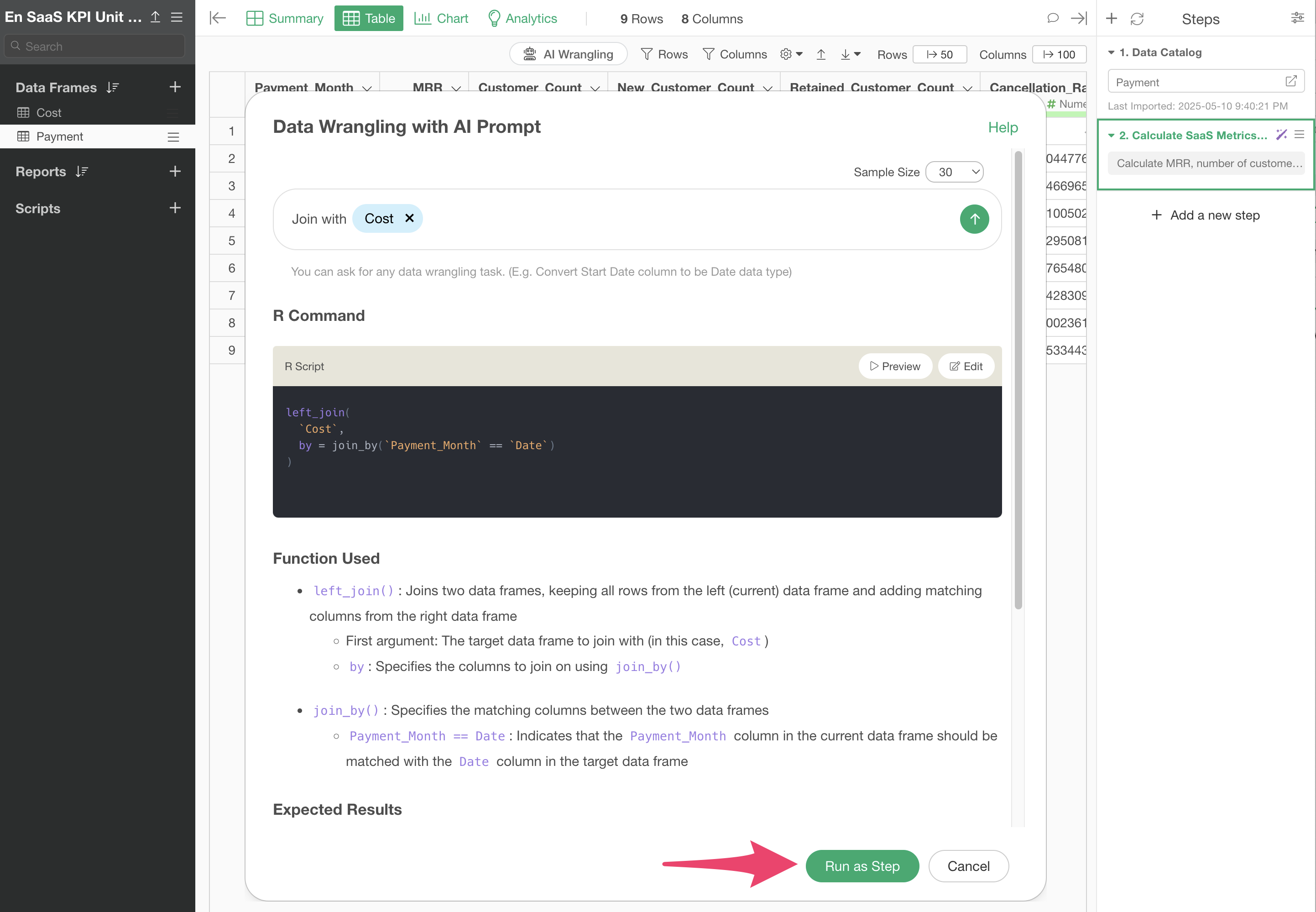
We have successfully joined the cost data.

Finally, we will calculate Unit Economics from the data we have prepared.

Click the “AI Wrangling” button. When the AI Prompt dialog appears, enter a prompt like the one below and run it:

Calculate Unit Economics

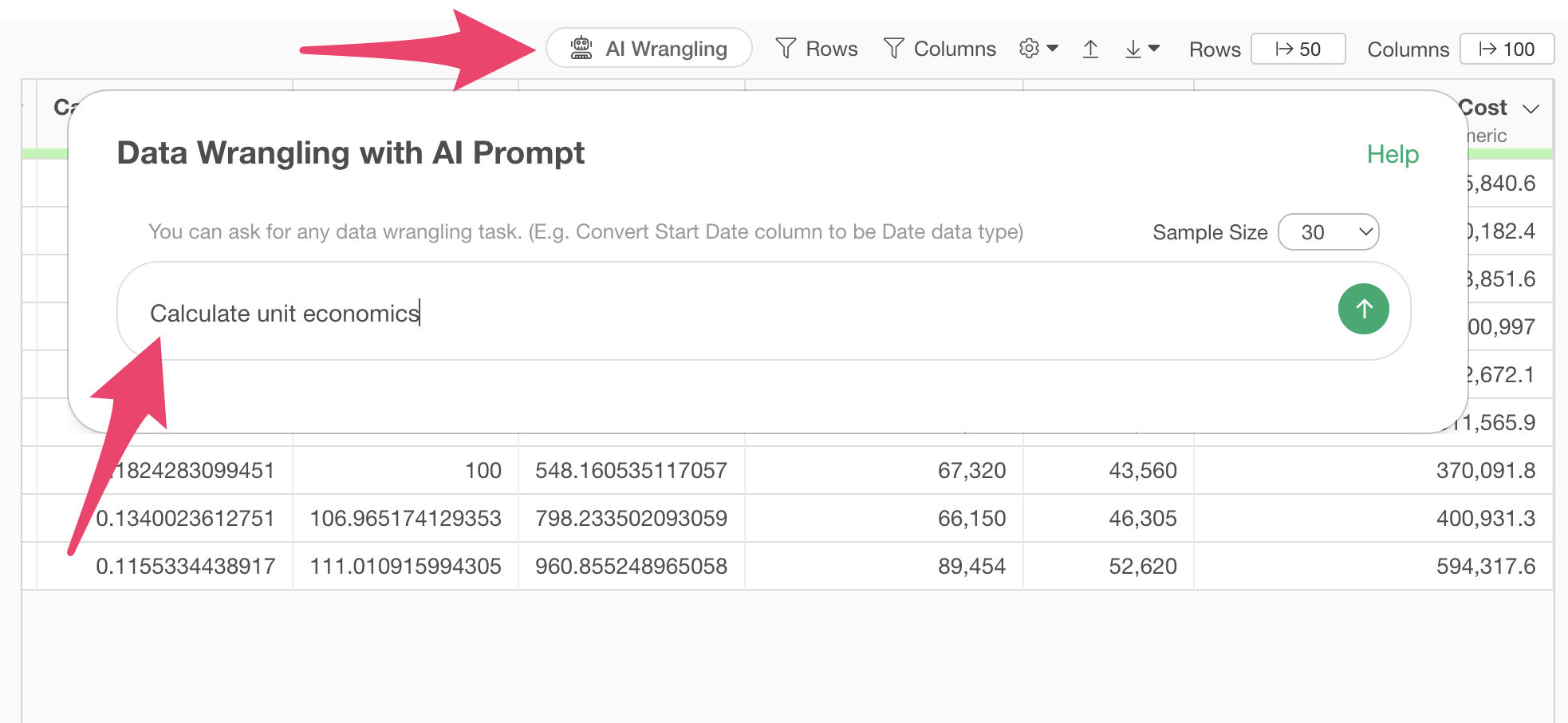
This will generate code to calculate Unit Economics (CLV / CAC) from CLV (Customer Lifetime Value) and newly generated CAC (Customer Acquisition Cost) column.

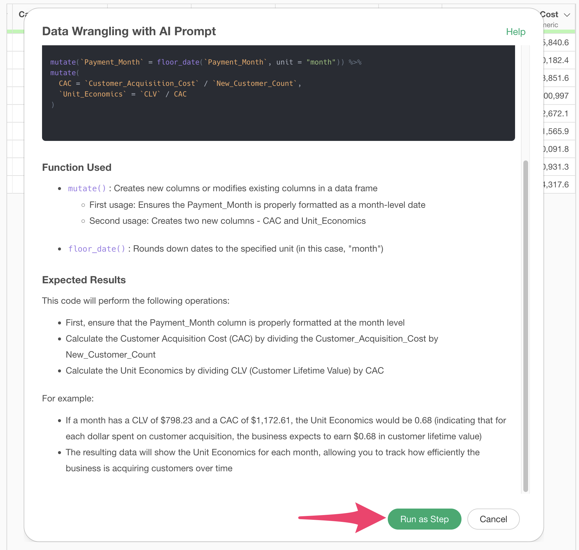
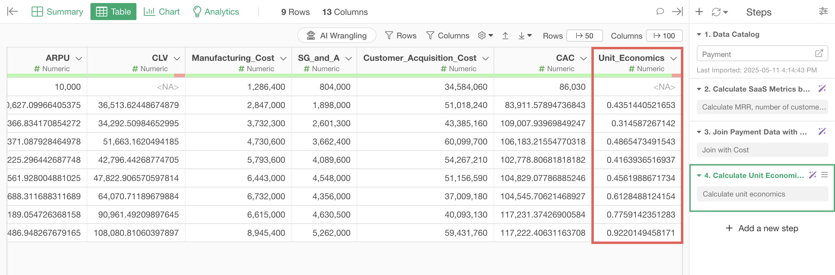
After checking the results, click the “Run as Step” button.

The step is added, and we have calculated Unit Economics.

Calculate Unit Economics with UI

Here I will introduce how to calculate Unit Economics using the UI.

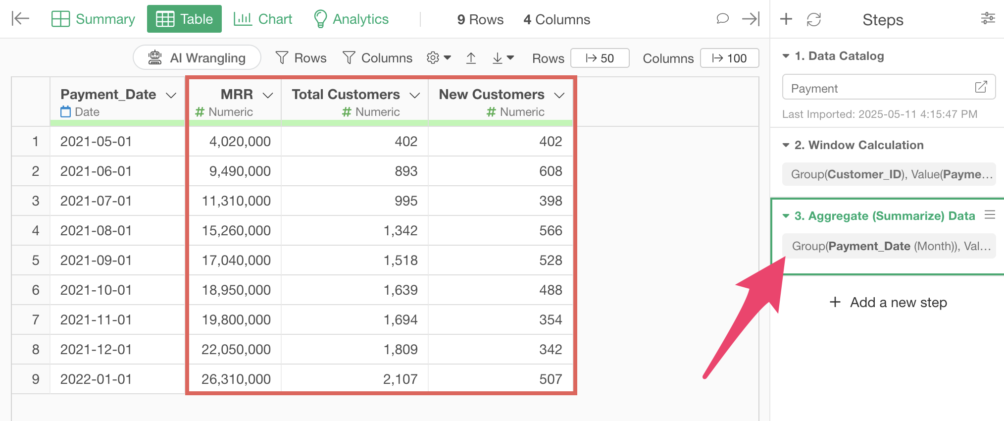
From the two datasets mentioned earlier, we will create a table like the following:

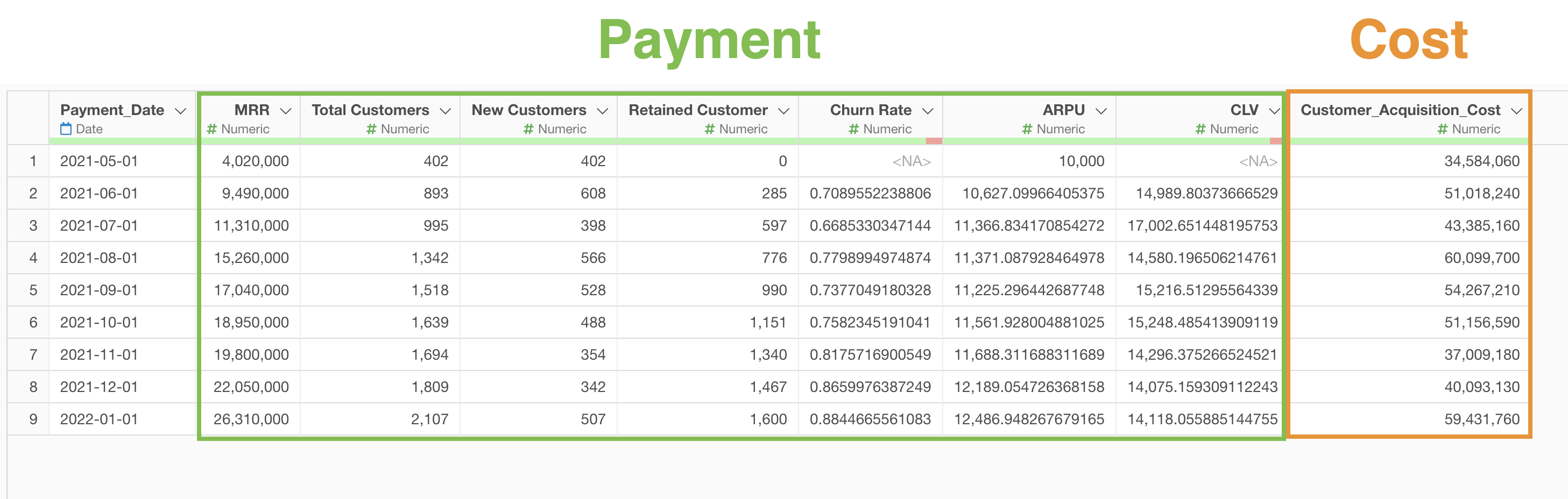
Once we create such a table, we will have the information necessary to calculate Unit Economics, so let’s first create the above table.

1. Aggregating MRR, Number of Customers, and Number of New Customers

MRR can be calculated by aggregating the total “Payment _Amount” by month, and the number of customers can be calculated by aggregating the number of unique customer IDs by month.

However, the number of new customers cannot be calculated just by aggregating payment data. If the original data has information about the number of payments, we can calculate the number of new customers by aggregating the unique number of customers who have made only one payment.

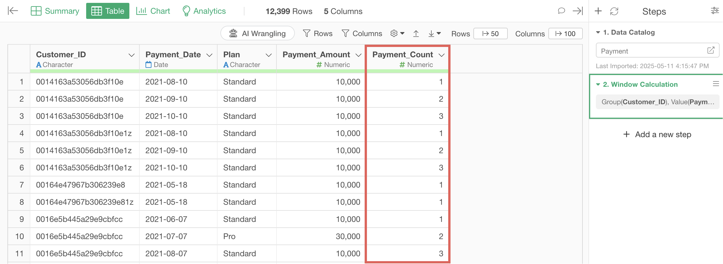
To calculate the number of payments in the payment data, select “Create Window Calculation”, “Dense Rank” and “Ascending” from the column header menu of the “Payment_Date” column.

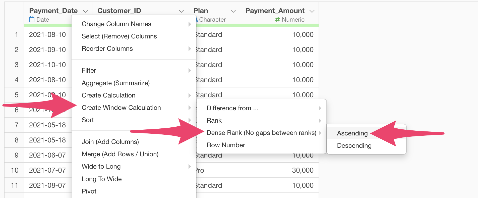
We do this to calculate the payment number by ranking payment dates in ascending order for each customer.

We select “Dense” as the ranking method to ensure that payments made on the same day, such as those due to upgrades, are not treated as separate payments.

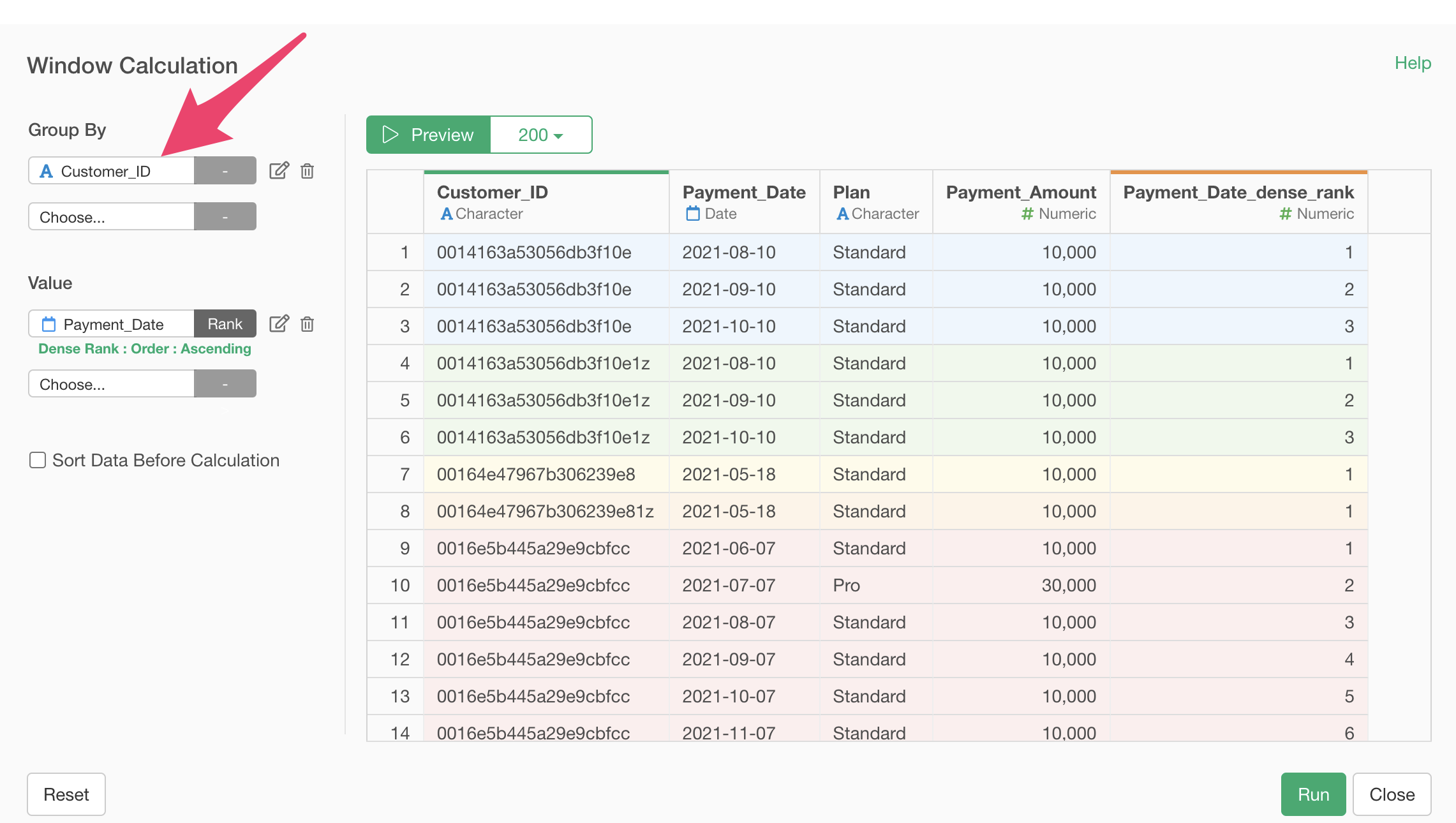
Since we want to calculate rankings for each customer, when the window calculation dialog opens, select “Customer_ID” for the group and click the preview button.

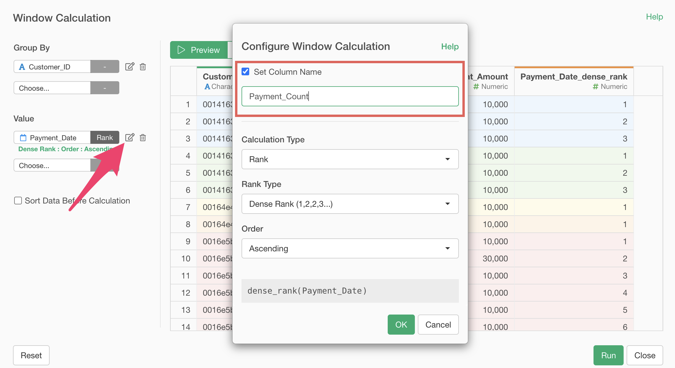
Finally, change the column name to “Payment_Count” and click the “Run” button.

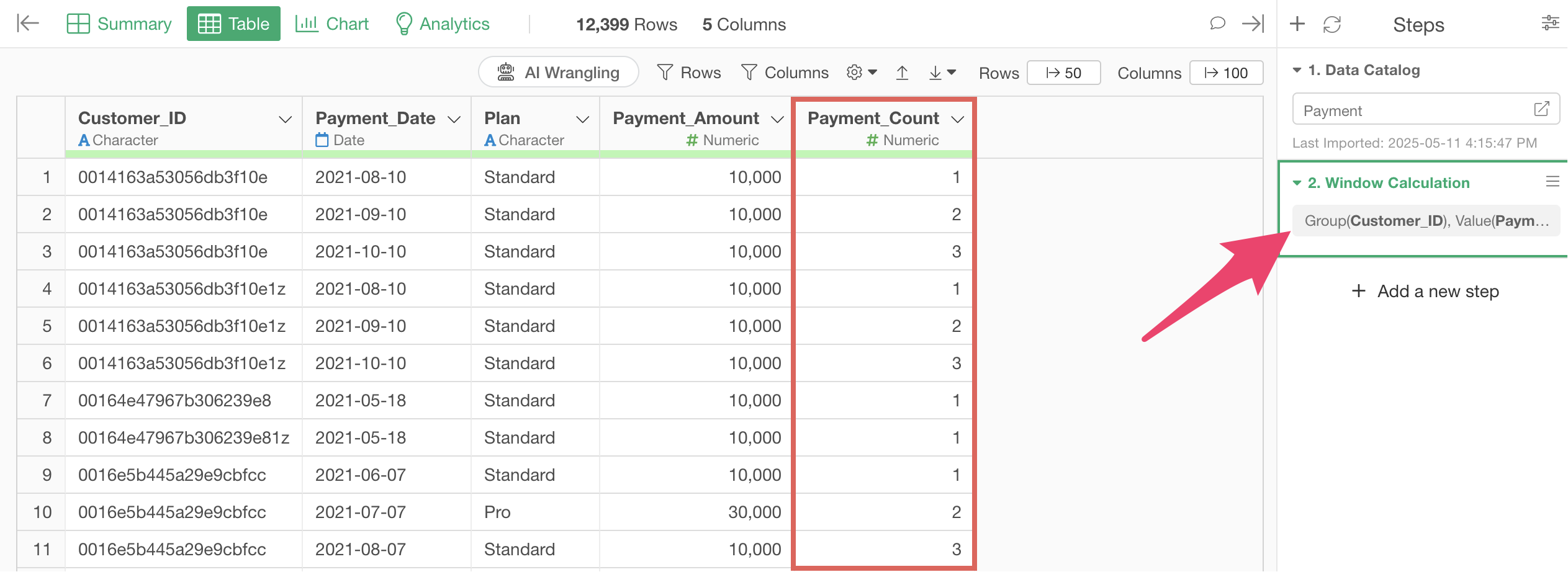
Now we have added payment number information to the payment data.

Next, we will aggregate MRR (Monthly Recurring Revenue). MRR is a metric needed to calculate ARPU, which is used in CLV calculation.

MRR is the monthly total of amounts paid by each user, so it can be easily calculated by computing the monthly payment amount.

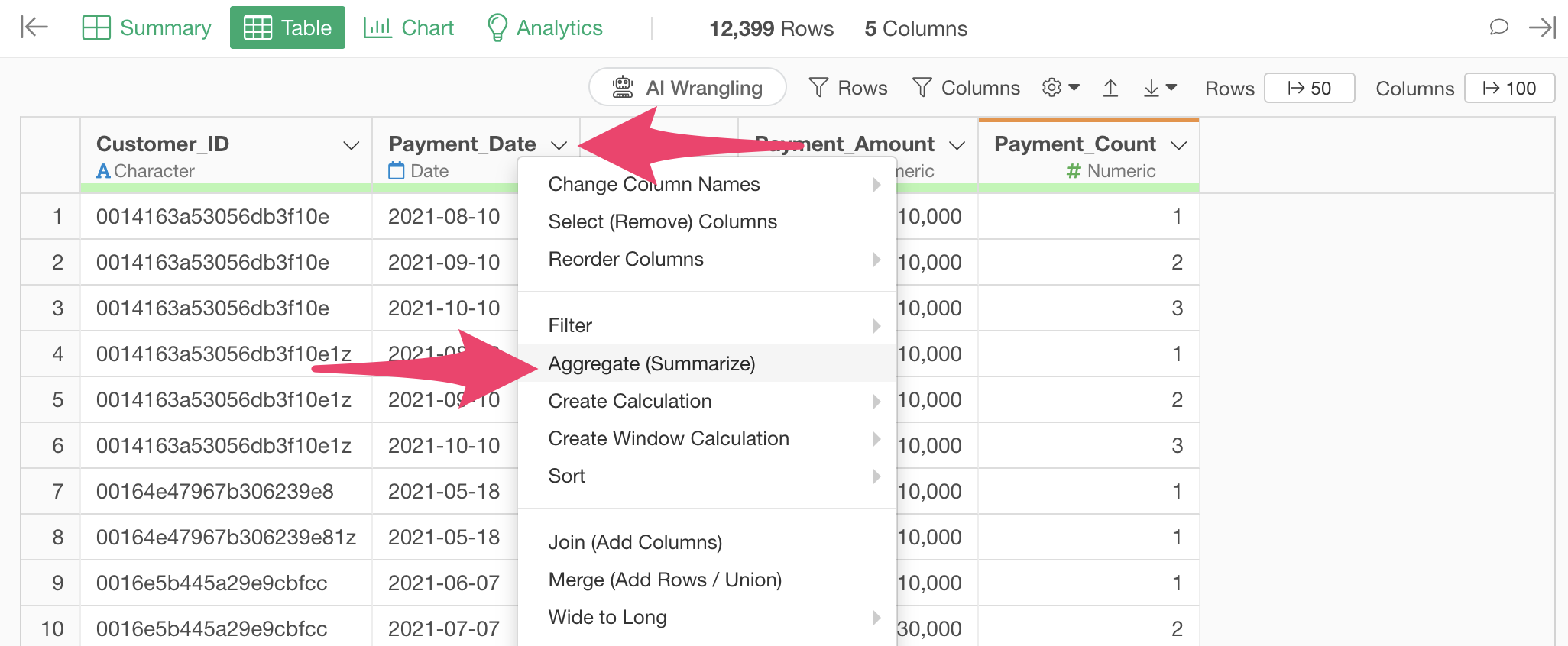
Select “Aggregate (Summarize)” from the column header menu of “Payment_Date”.

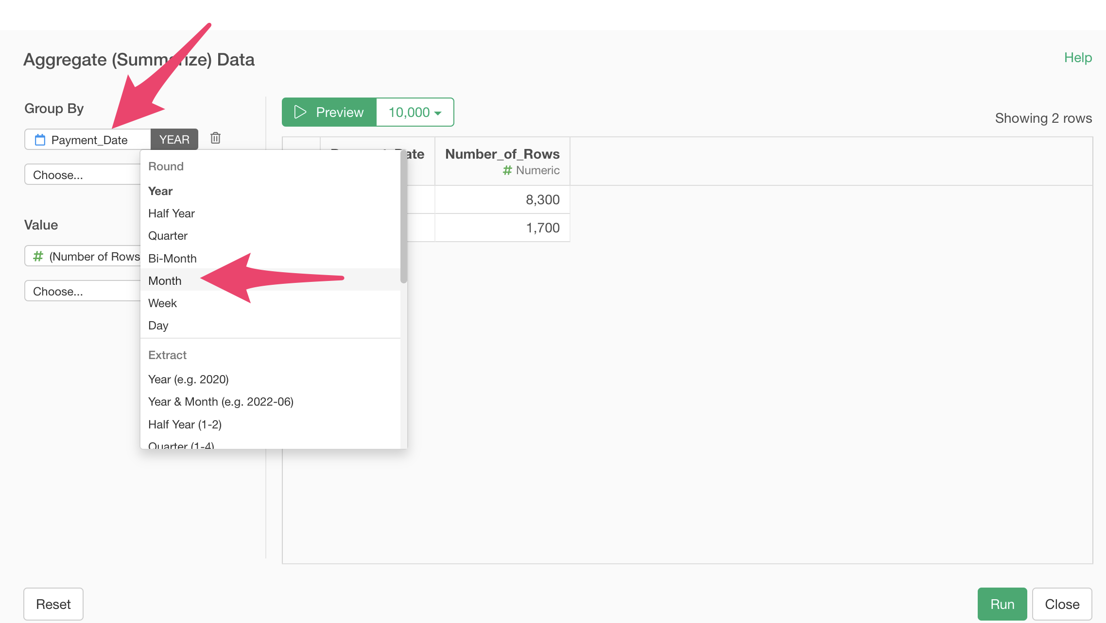
When the aggregation dialog appears, select “Payment_Date” for the group and choose “Month” with truncation for the date unit.

Next, select “Payment_Amount” for the value and SUM as the aggregation function.

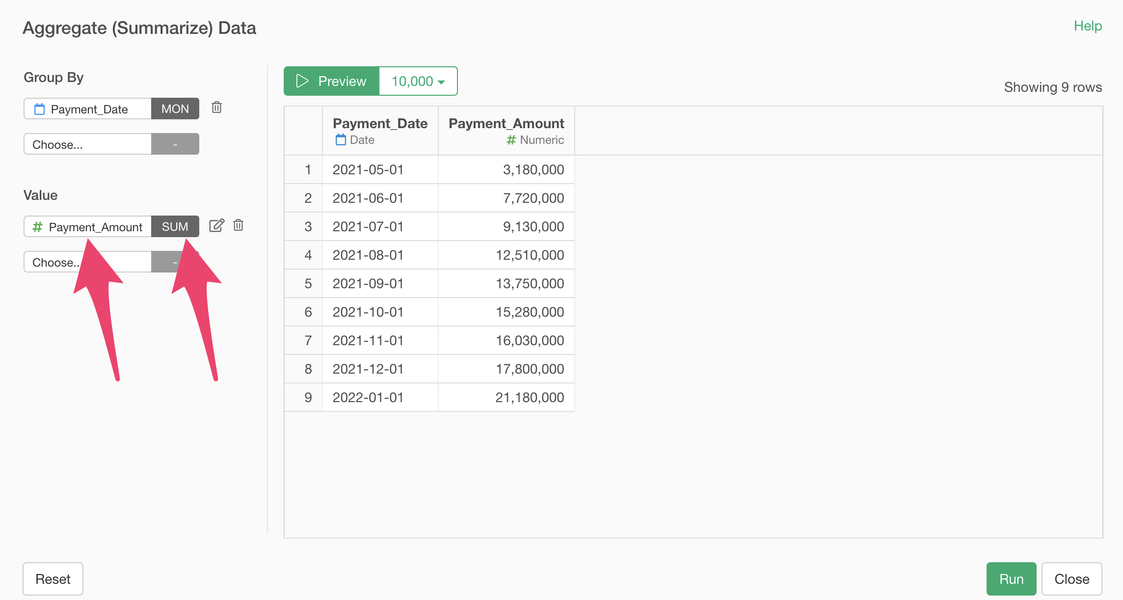
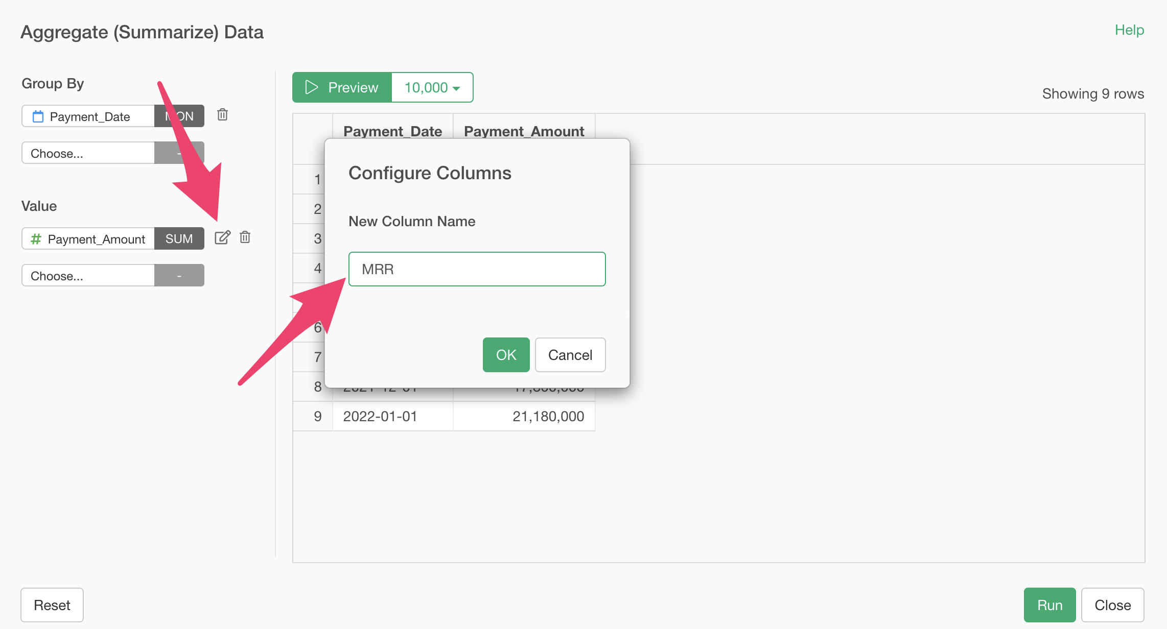
Finally, change the column name to “MRR” and click the preview button.

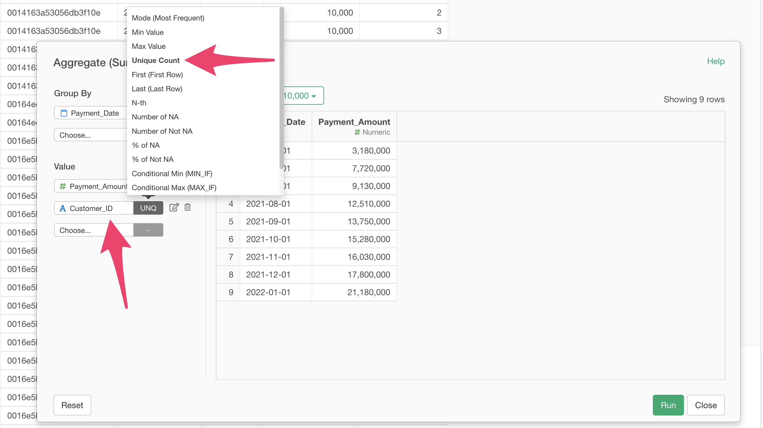
Next, we will aggregate the number of customers. The number of customers is a metric needed to calculate ARPU, which is used in CLV calculation.

In the aggregation dialog, select “Customer_ID” for the value and “Unique_Count” for the aggregation function.

Next, click the edit icon to change the new column name to “Total Customers” and click the “OK” button.

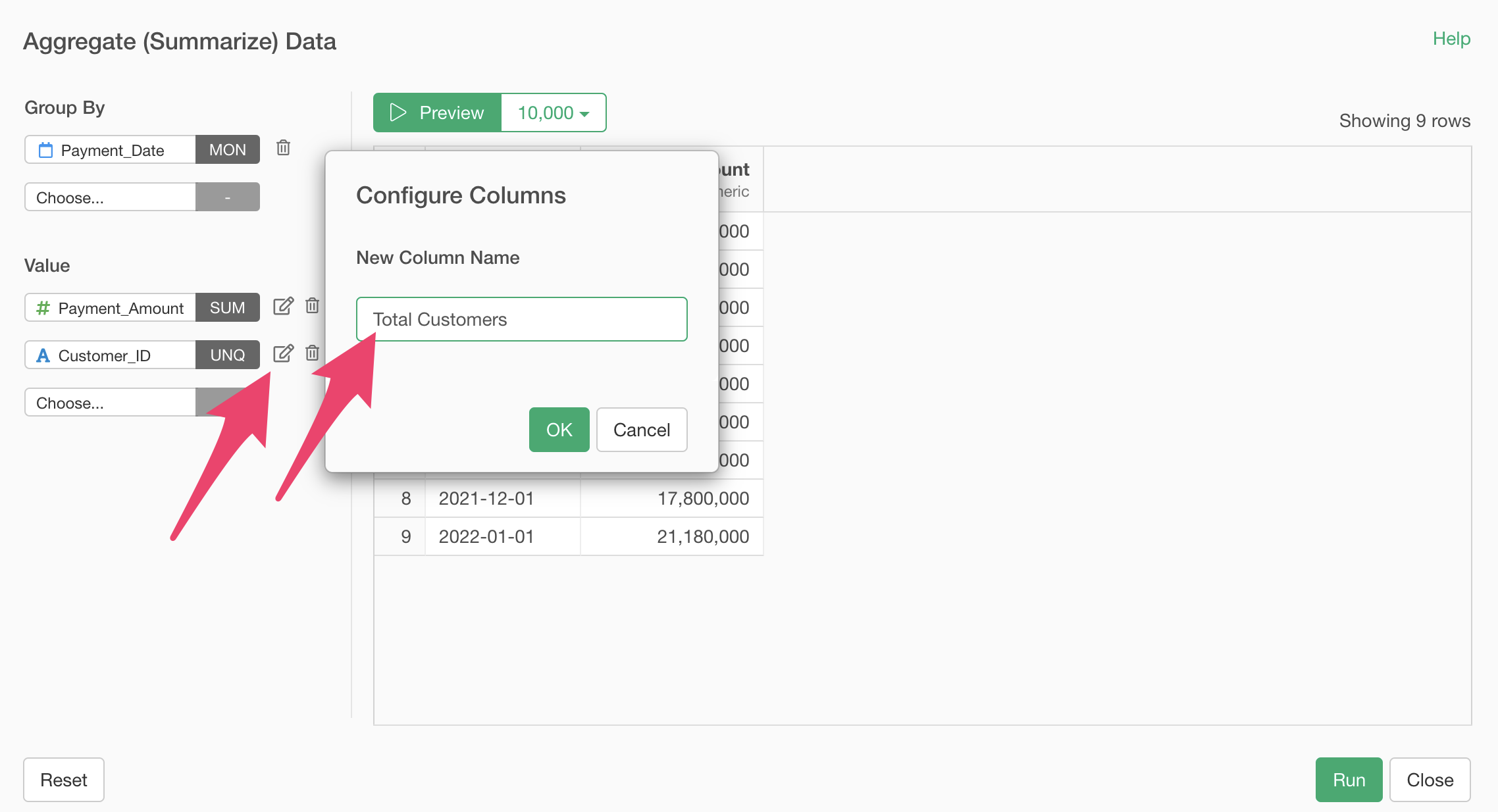
We are now ready to aggregate the number of customers.

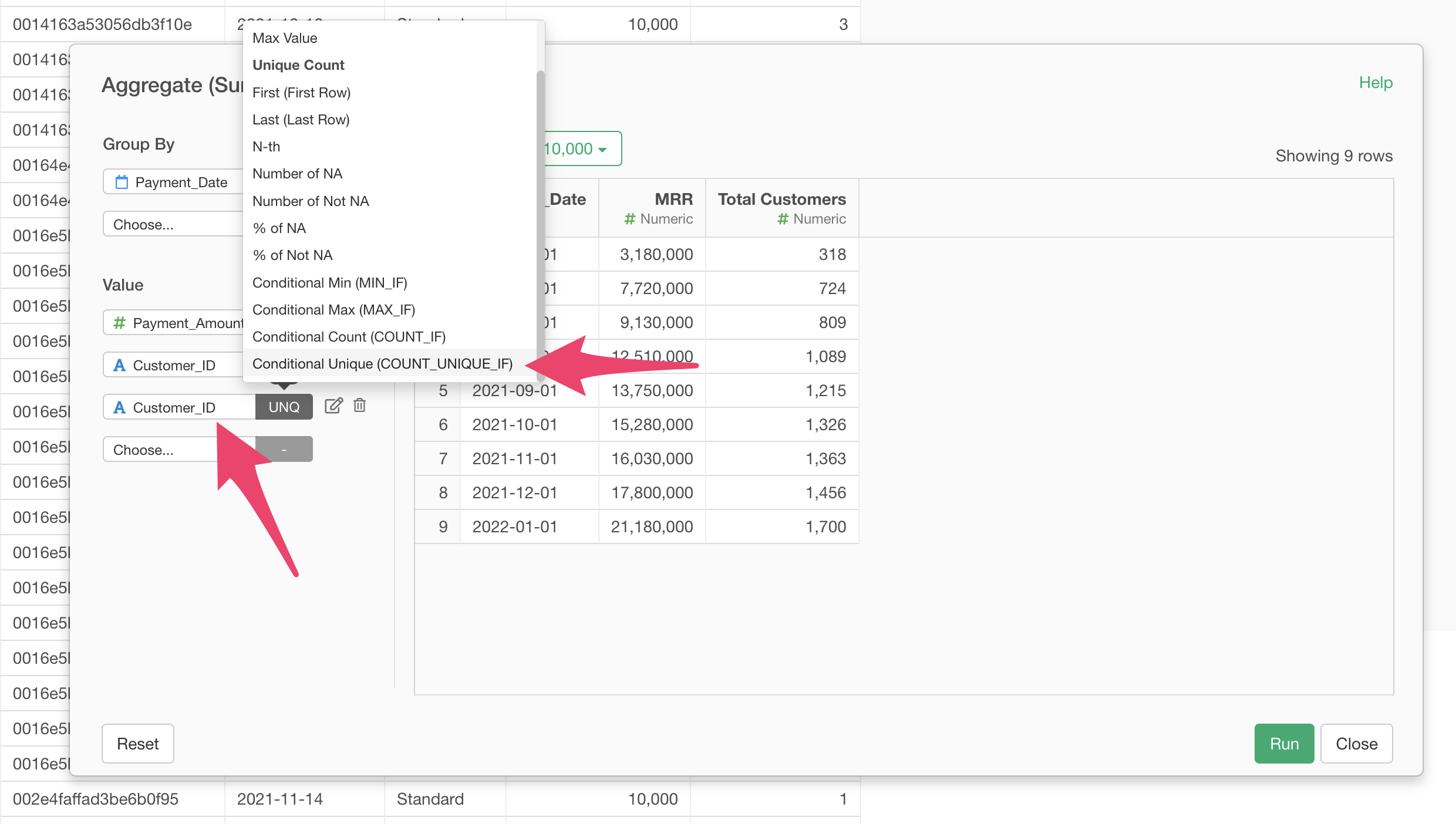
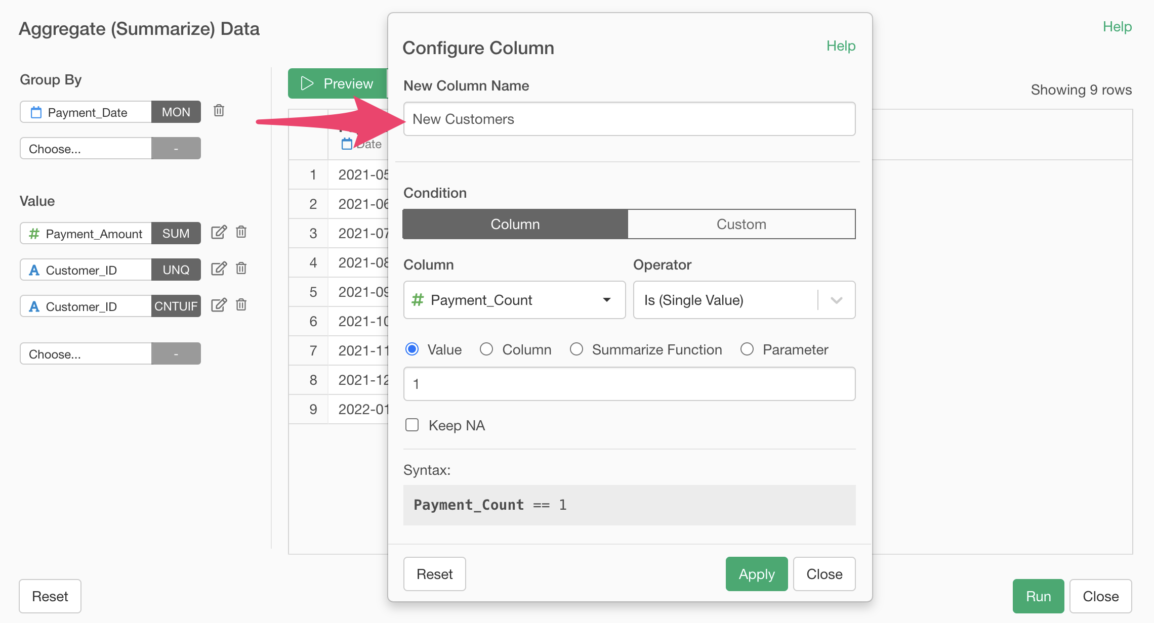
Finally, we will aggregate the number of new customers based on the payment number. The number of new customers is an essential metric for calculating CAC (Customer Acquisition Cost) .

Select “Customer_ID” for the value and “Conditional Unique (COUNT_UNIQUE_IF)” for the aggregation function.

When the “Configure Column” dialog appears to set conditions, enter “Payment_Count” for the column, “Is” for the operator, and “1” for the value.

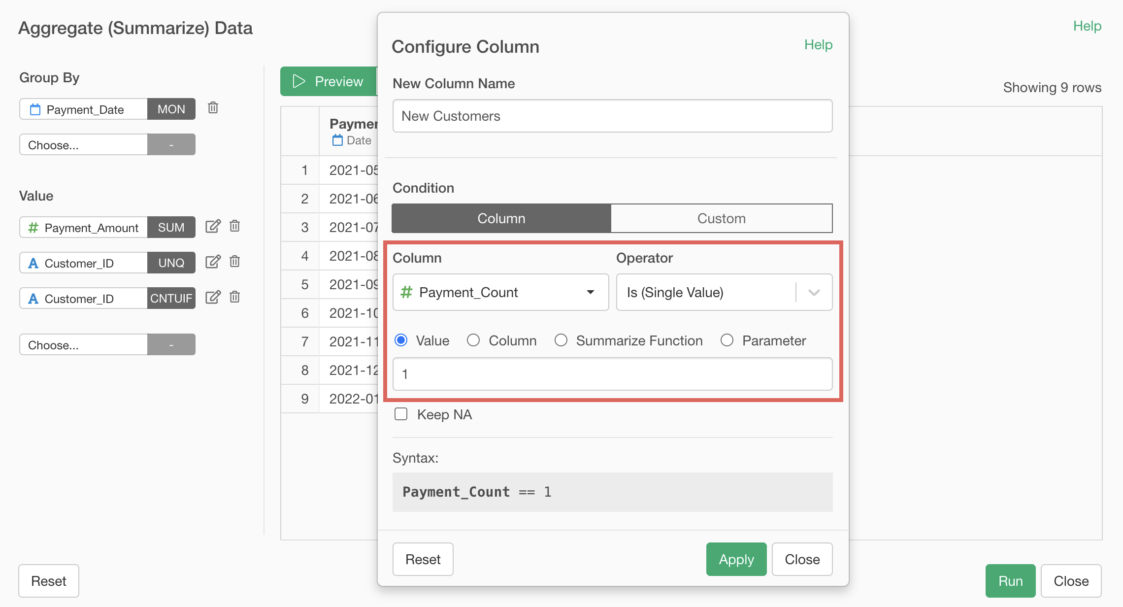
This setting allows us to aggregate the unique number of Customer IDs with a “Payment_Count” of 1.

Next, enter “New Customers” as the new column name and click the “Run” button.

We have successfully aggregated MRR, number of customers, and number of new customers.

2. Calculating Number of Continuing Customers and Churn Rate

Next, we will calculate the number of continuing customers to calculate the churn (cancellation) rate.

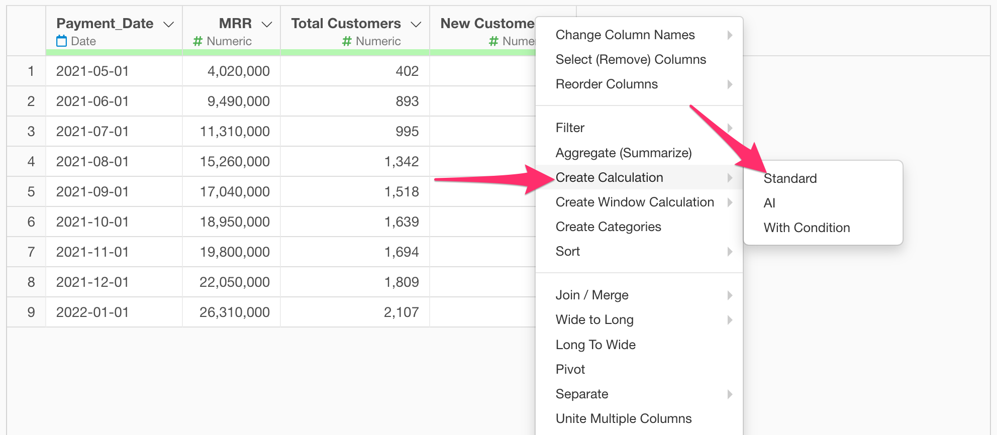
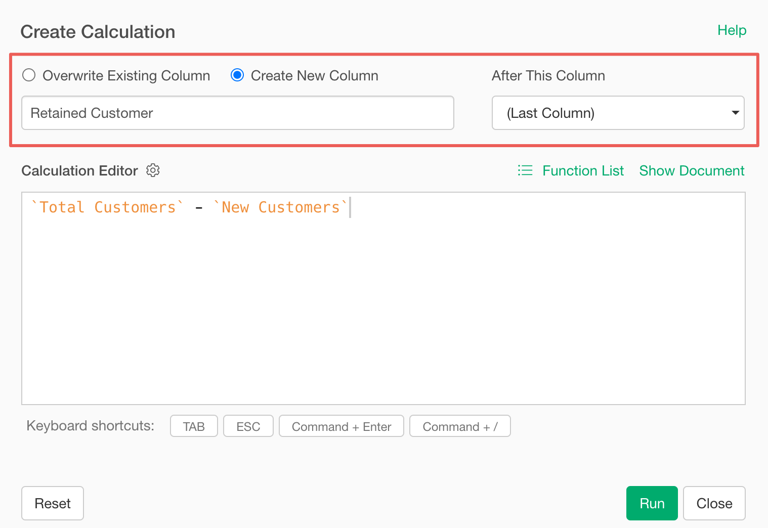
Select “Create Calculation” and “Standard” from the column header menu of “Total Customers”.

When the create calculation dialog opens, enter `Total Customers` - `New Customers` in the calculation editor.

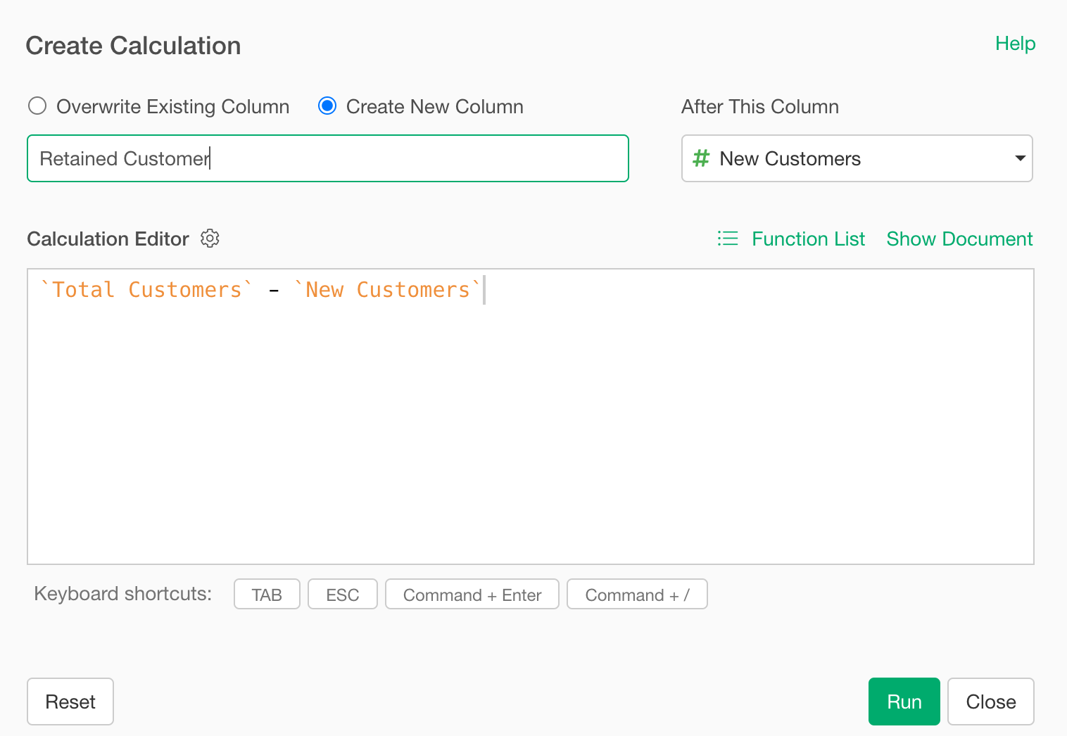
Confirm that “Create New Column” is checked, set the column name to “Retained Customer”, set ” After This Column” to “Last Column”, and click the “Run” button.

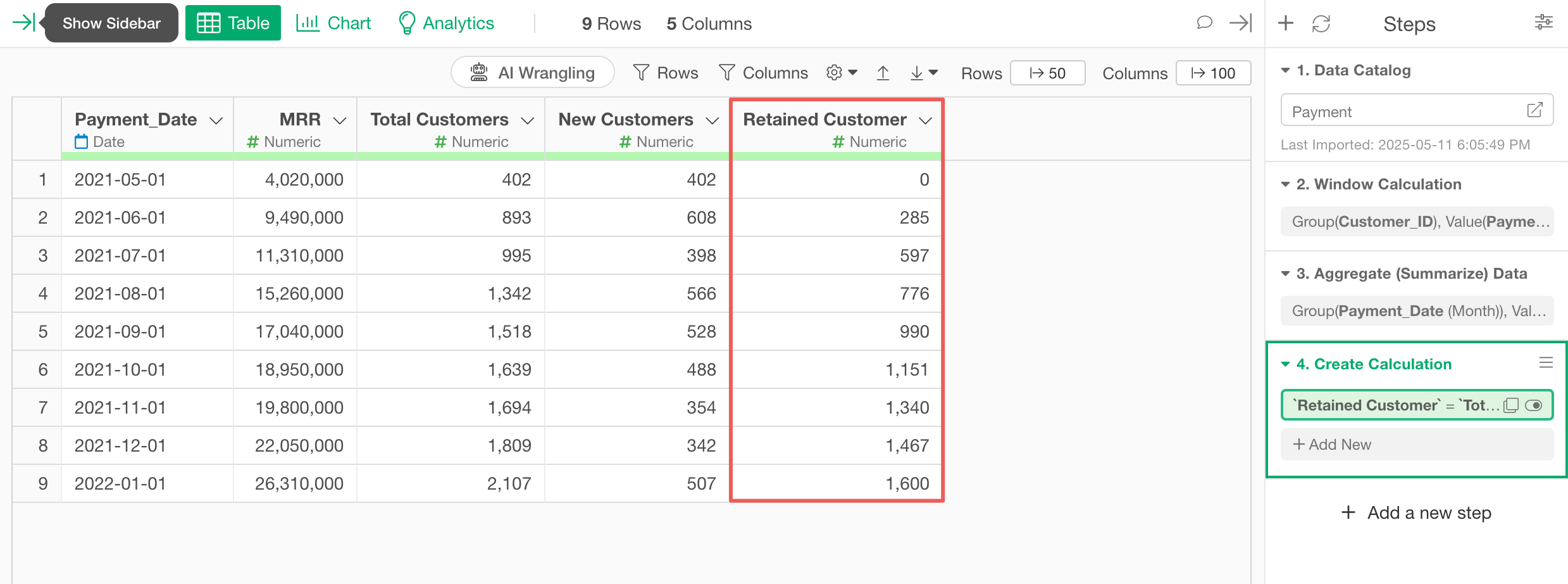
We have created a new column “Retained Customer”.

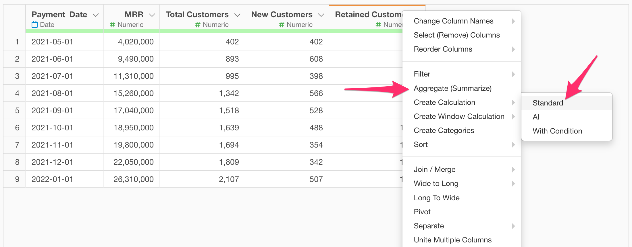
Next, we will calculate the churn rate.

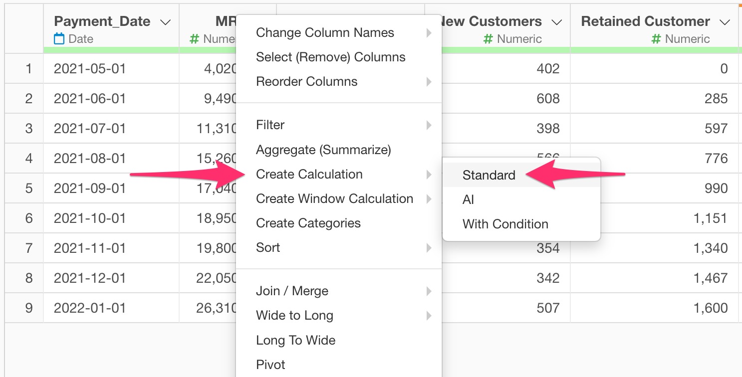
Select “Create Calculation” and “Standard” from the column header menu of “Retained Customer”.

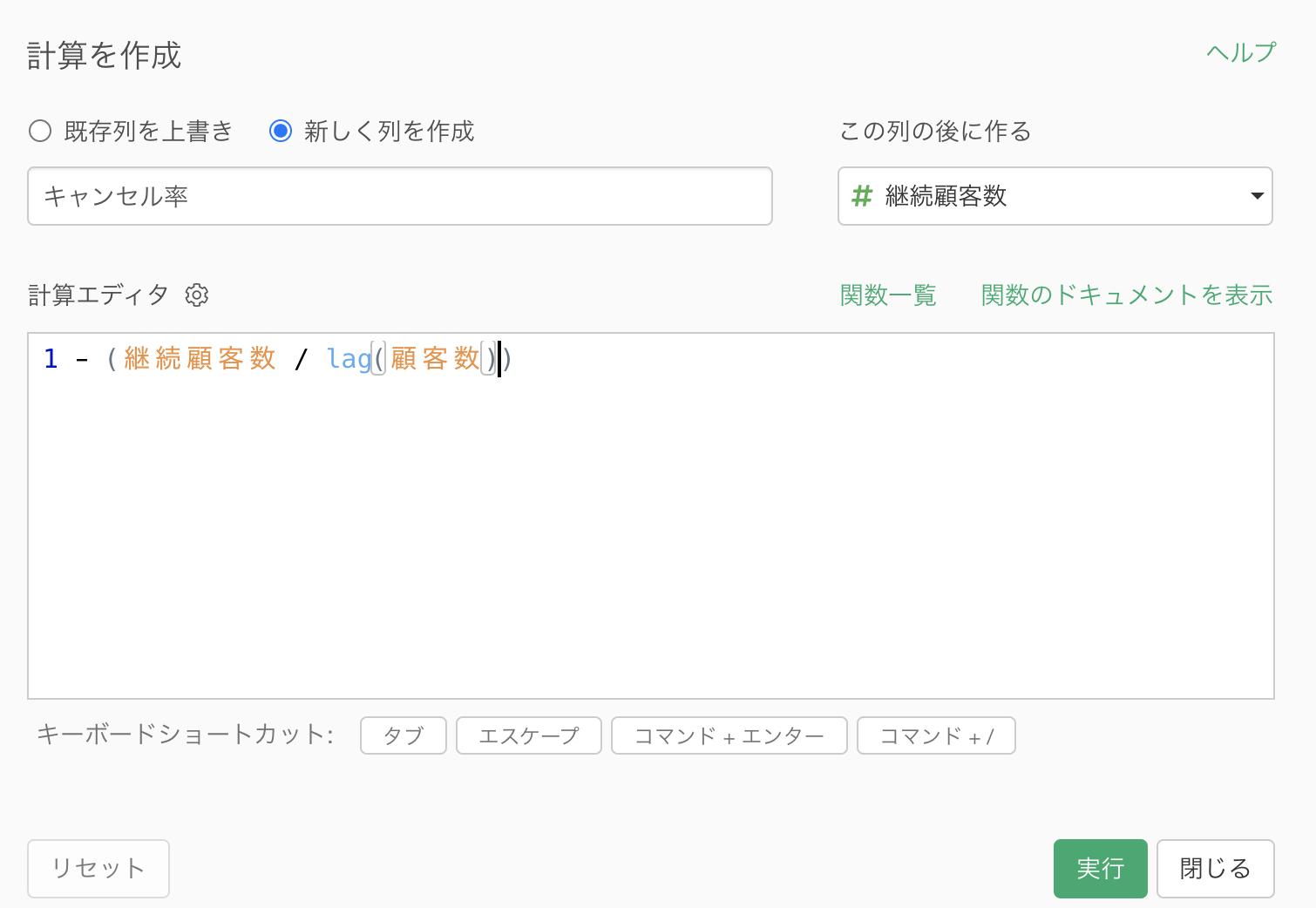
When the “Create Calculation” dialog appears, enter `Retained Customer` / `Total Customers` in the calculation editor.

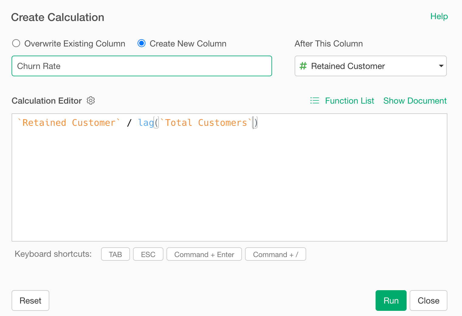
Note that the lag function retrieves the value from the previous row, so the calculation `Retained Customer` / lag(`Total Customers`) calculates the proportion of customers from the previous month who continued the service this month.

However, since the proportion of customers who continued the service is the retention rate, to calculate the churn rate (which is the inverse of retention rate), change the content of the ∅calculation editor to 1 - (`Retained Customer` / lag(`Total Customers`)).

Confirm that “Create New Column” is checked, set the column name to “Churn Rate”, set “After this column” to “Last Column”, and click the “Run” button.

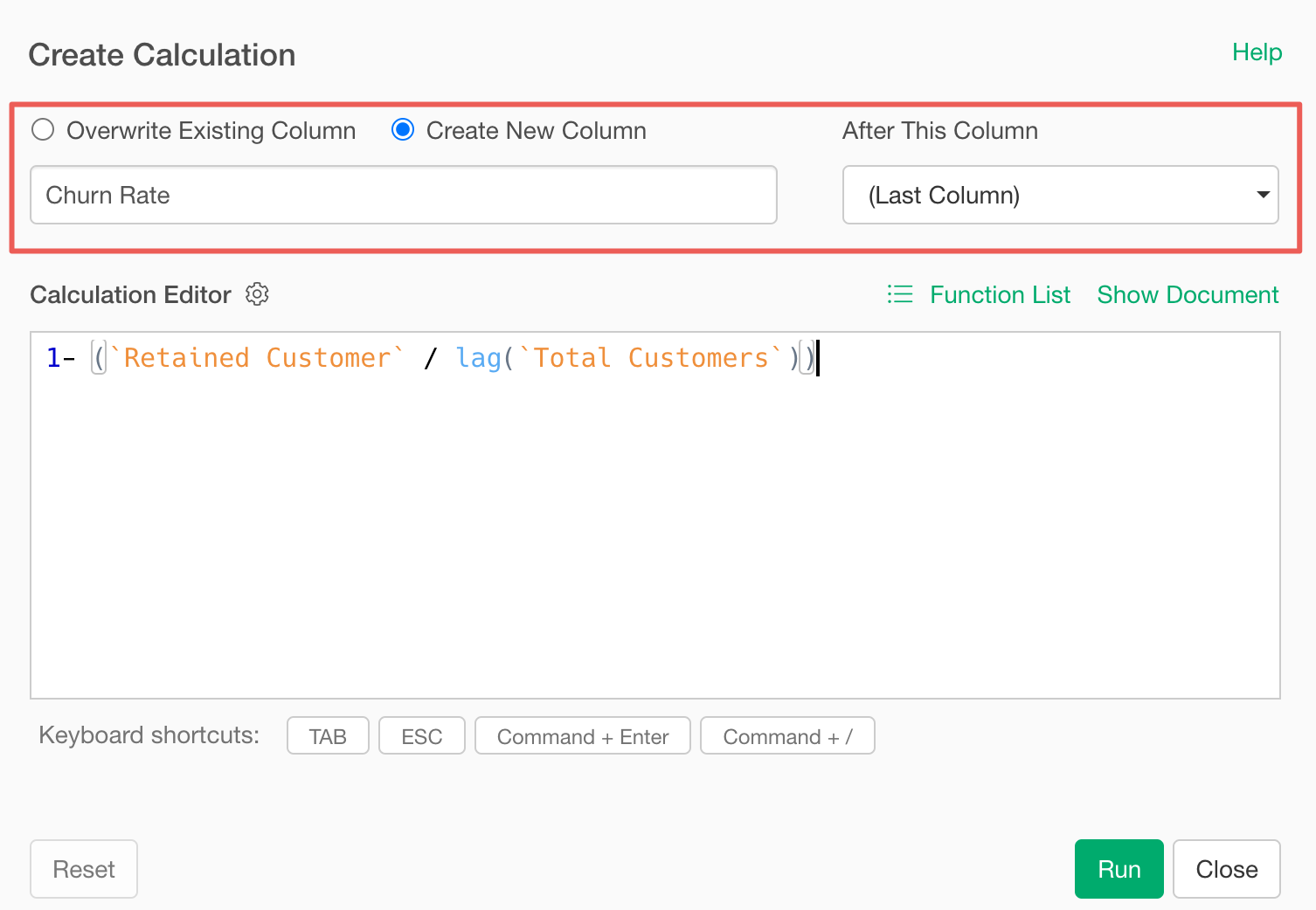
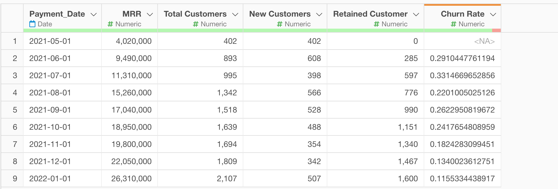
We have calculated the churn rate.

3. Calculating ARPU and CLV

Next, we will calculate ARPU and CLV.

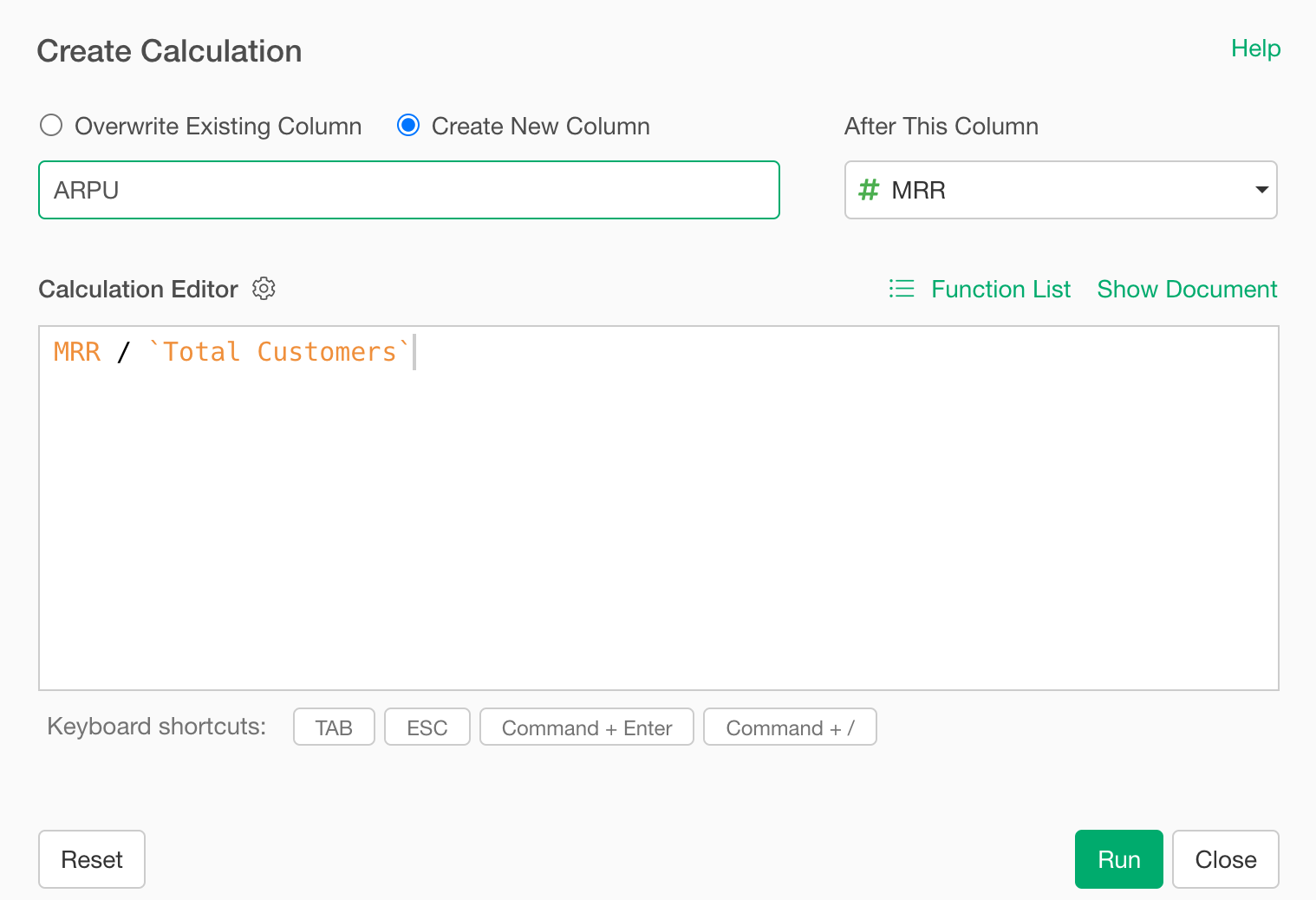
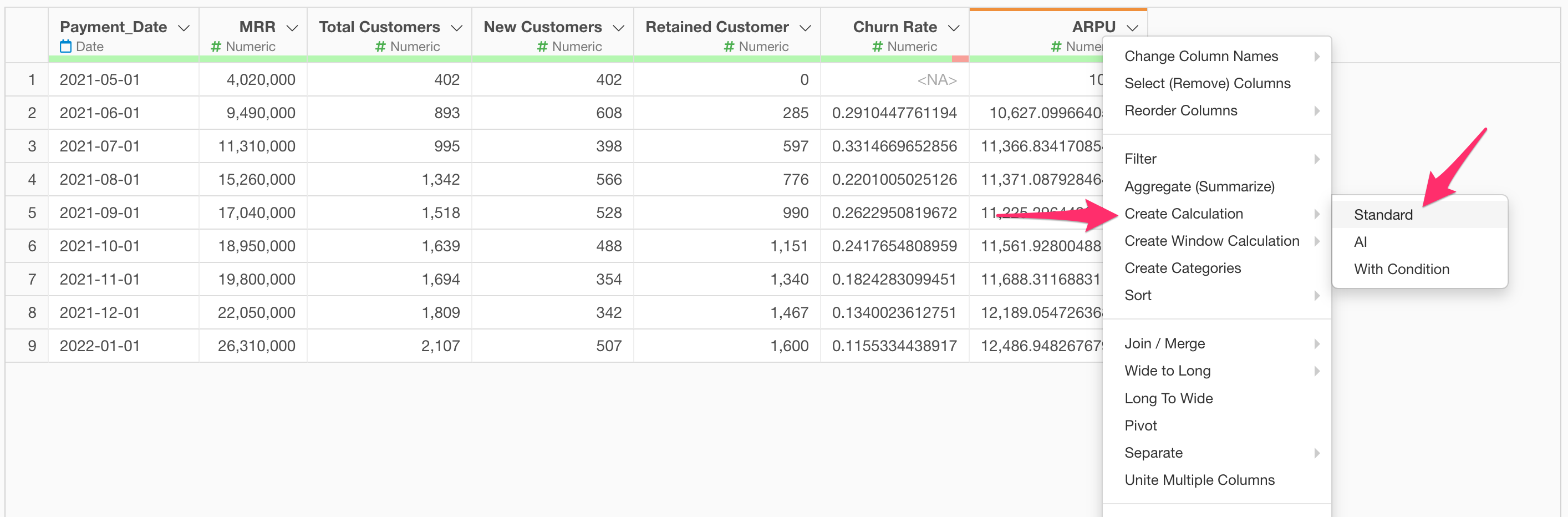
Select “Create Calculation” and “Standard” from the column header menu of MRR.

When the create calculation dialog opens, enter MRR / `Total Customers` in the calculation editor.

Finally, confirm that “Create New Column” is checked, set the column name to “ARPU”, change “After this column” to the last column, and click the “Run” button.

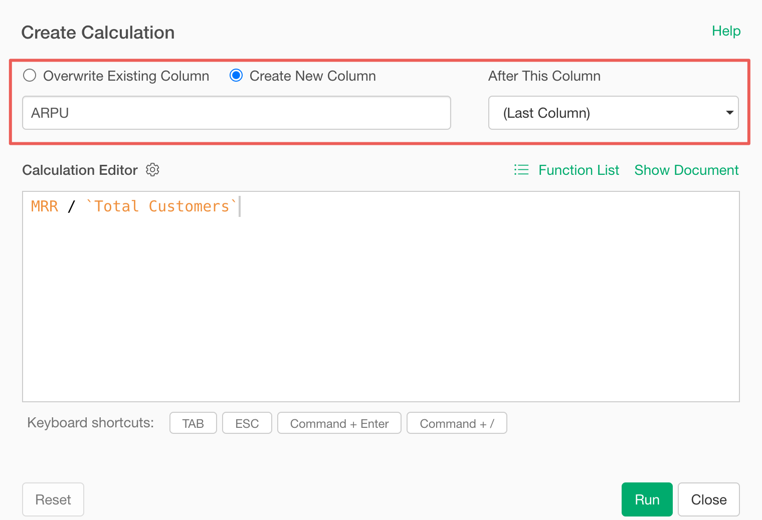
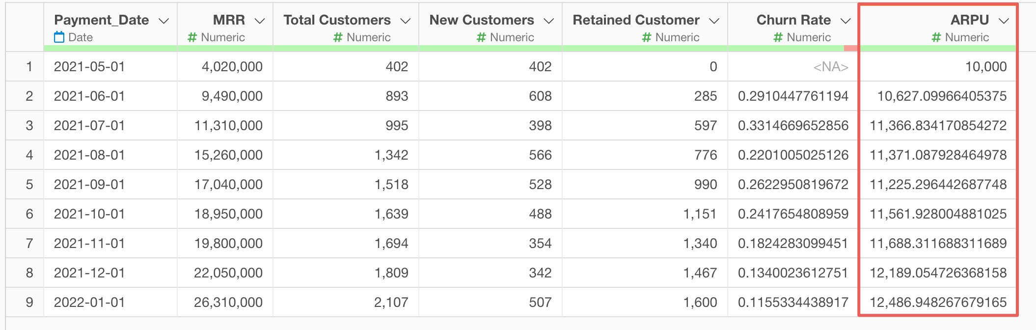
We have calculated ARPU.

Next, we will calculate CLV. While it is preferable to calculate CLV (Customer Lifetime Value) using survival curves for accurate calculation, this time we will use the following simplified formula to calculate CLV. (For details on how to calculate CLV using survival curves and why CLV can be calculated with the formula below, please check here)

\[\begin{aligned} \text{CLV } = \left( \frac{1}{\text{Churn Rate}} \right) \times \text{ARPU} \end{aligned}\]

Therefore, select “Create Calculation” and “Standard” from the column header menu of “Churn Rate”.

When the create calculation dialog opens, enter (1 / `Churn Rate`) * ARPU in the calculation editor.

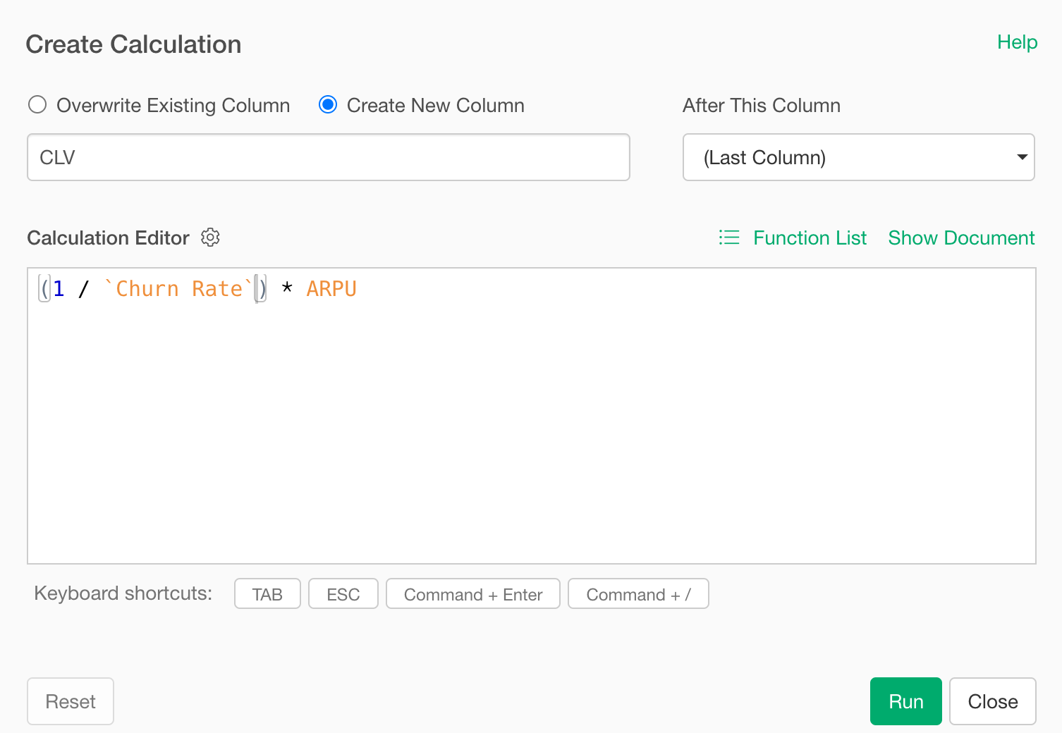
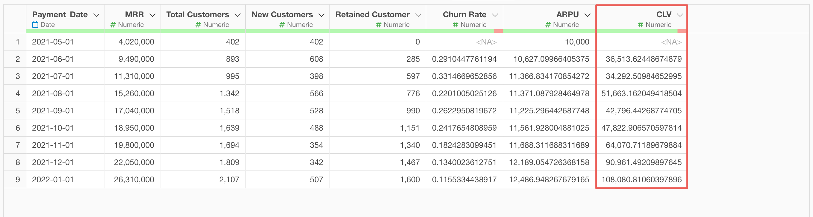
Confirm that “Create New Column” is checked, set the column name to “CLV”, change “After this column” to the last column, and click the “Run” button.

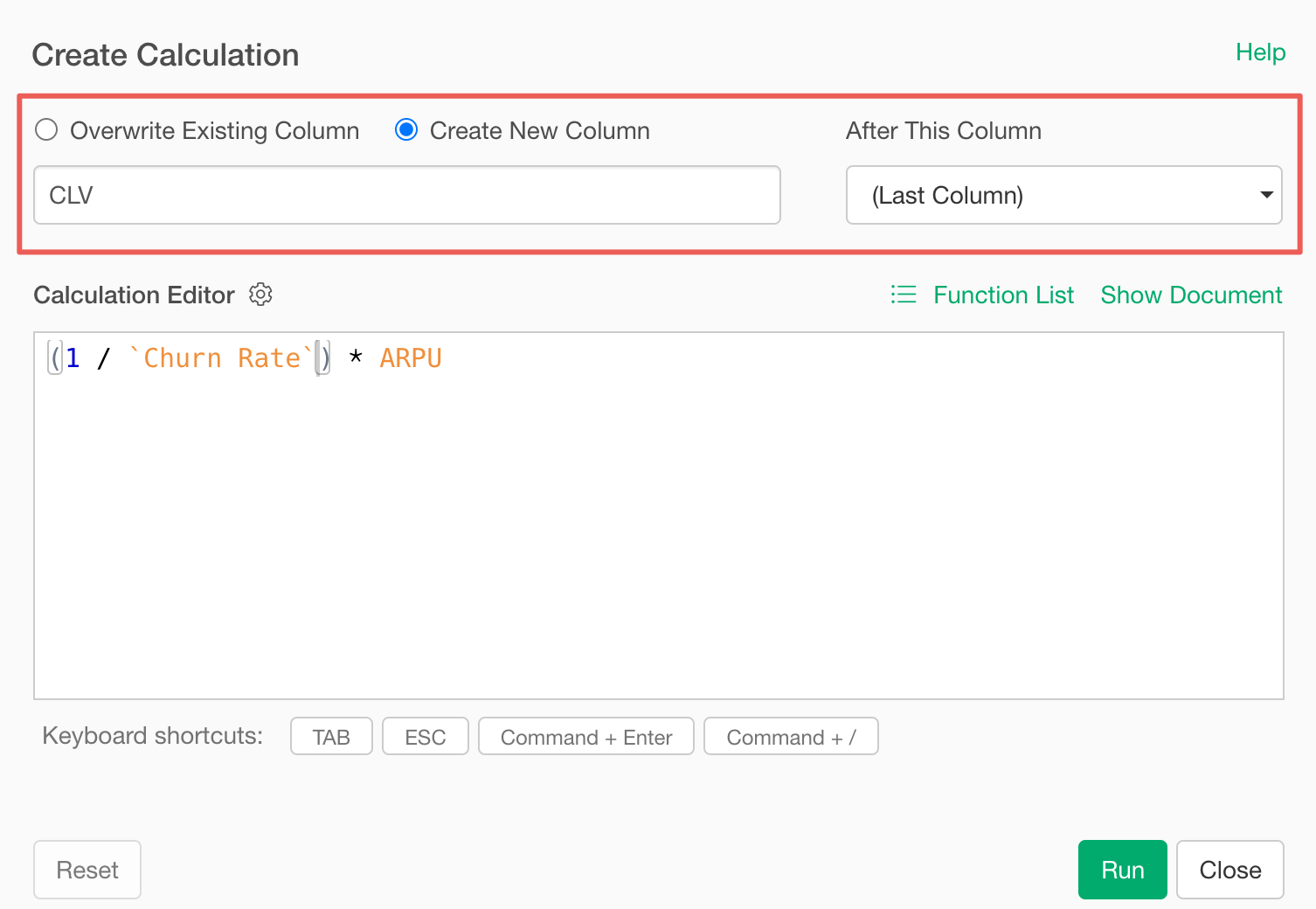
We have calculated CLV.

4. Joining Cost Data

Next, we will join the cost information to the data we have aggregated.

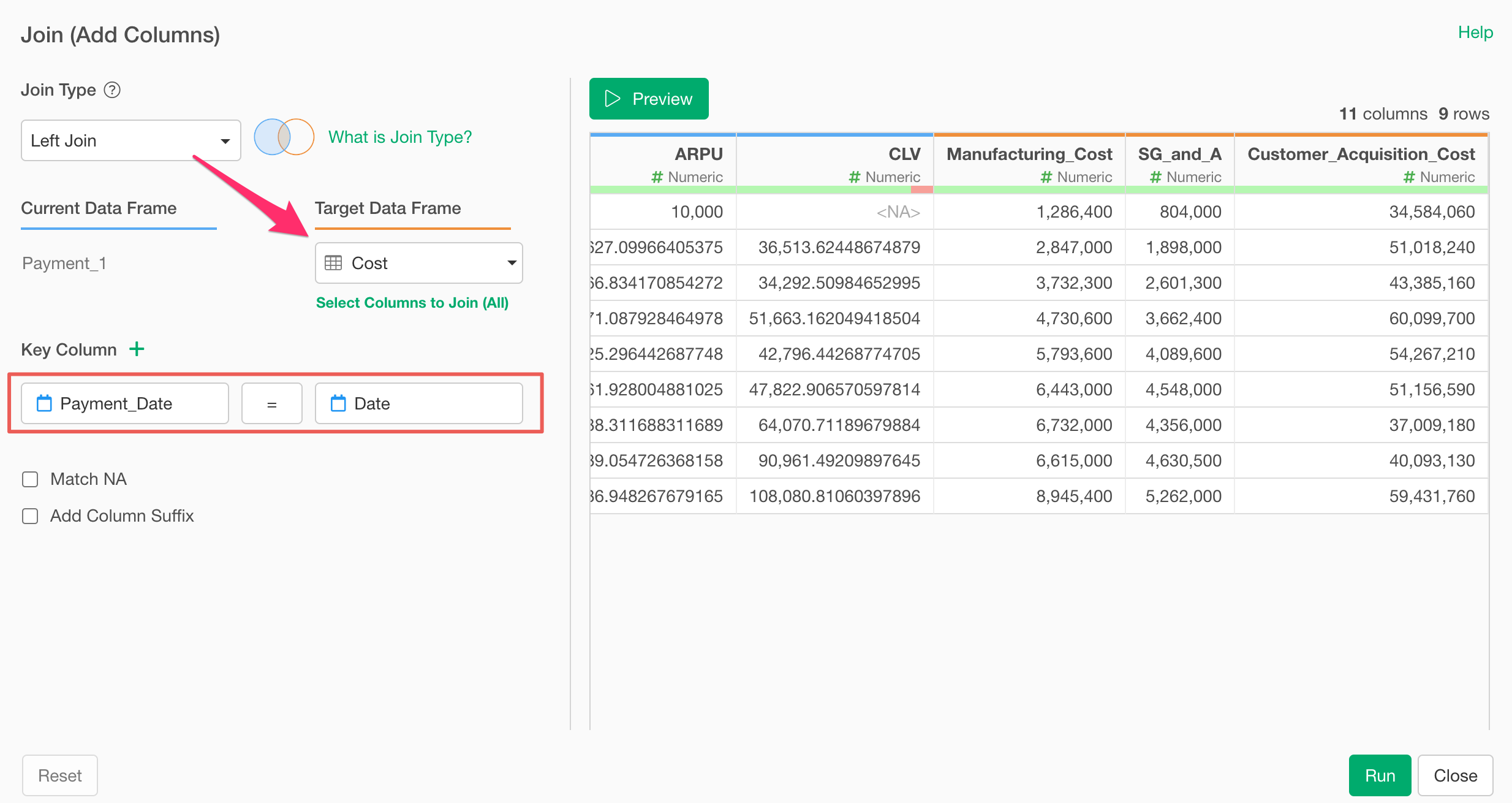
Select “Join (Add Columns)” from the column header menu of “Payment_Date”.

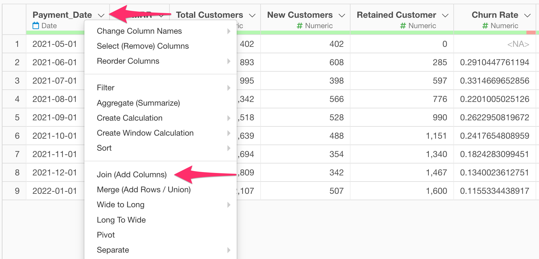
When the join dialog opens, select the cost data for “Target Data Frame”, select “Date” for the key column, and click the “Run” button.

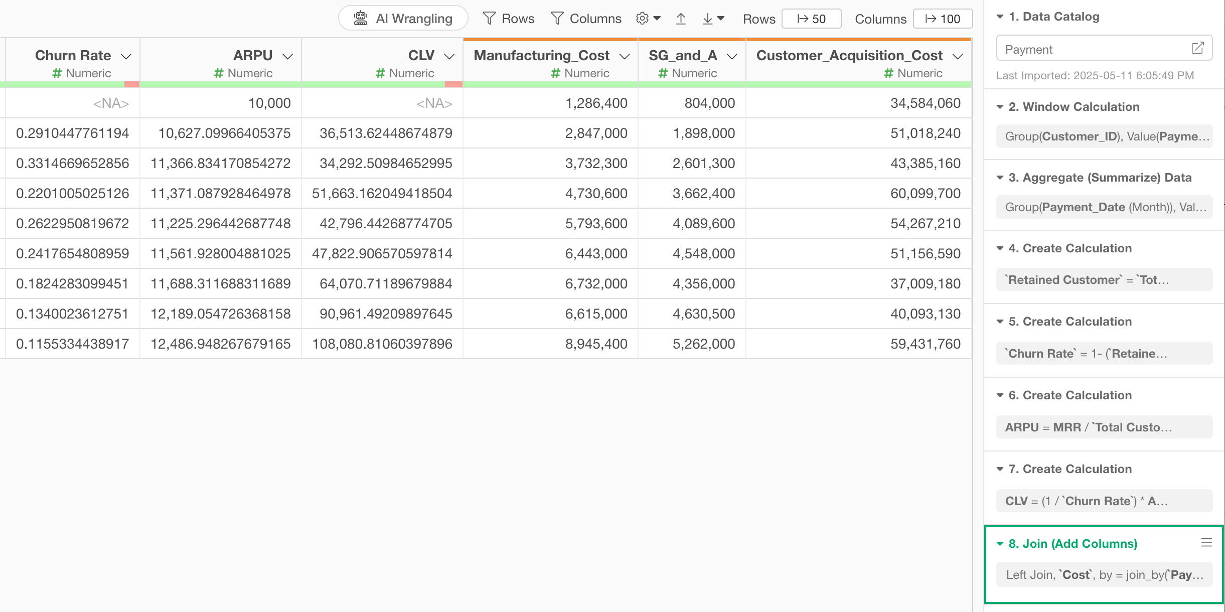
Now we have created the data needed to calculate Unit Economics.

5. Calculating Unit Economics

Finally, we will calculate Unit Economics.

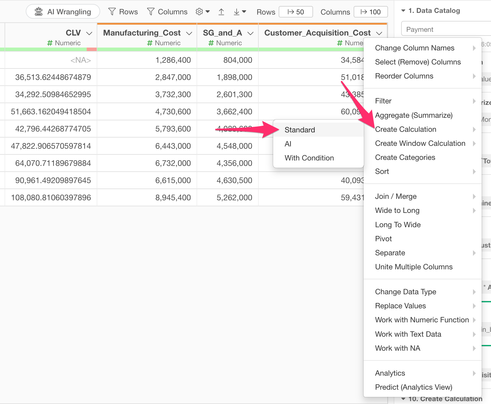
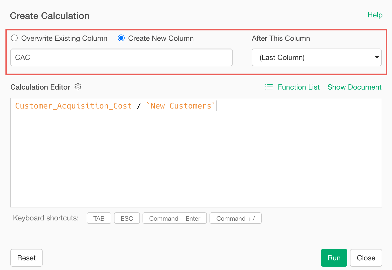
First, to calculate CAC (Customer Acquisition Cost), select “Create Calculation” and “Standard” from the column header menu of “Customer_Acquisition_Cost”.

When the create calculation dialog opens, enter Customer_Acquisition_Cost / `New Customers` in the calculation editor.

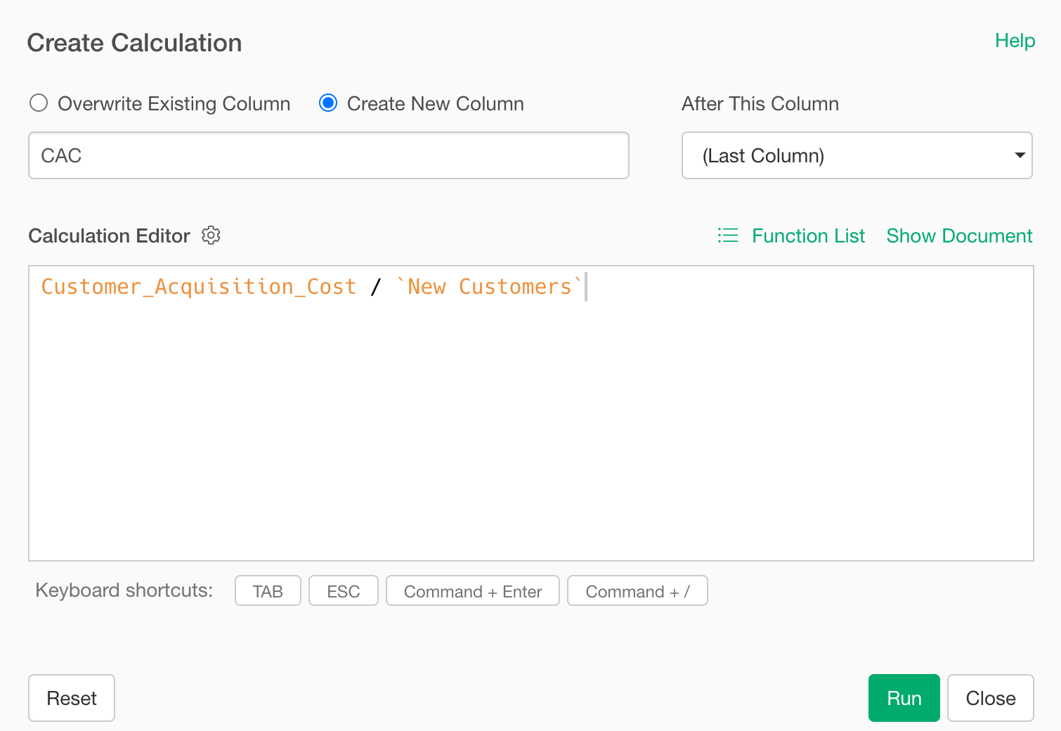
Confirm that “Create New Column” is checked, set the column name to “CAC”, set “After This Column” to “Last Column”, and click the “Run” button.

We have calculated CAC.

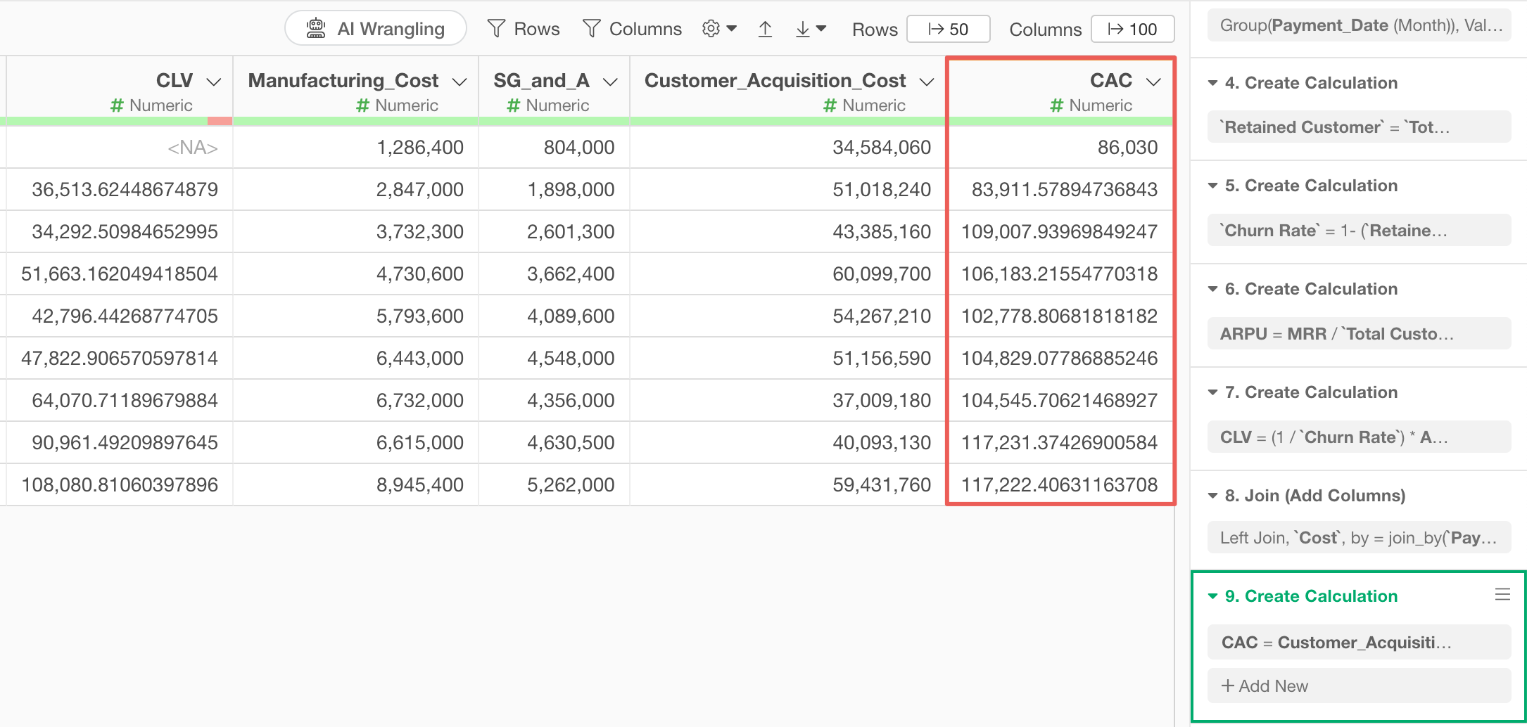
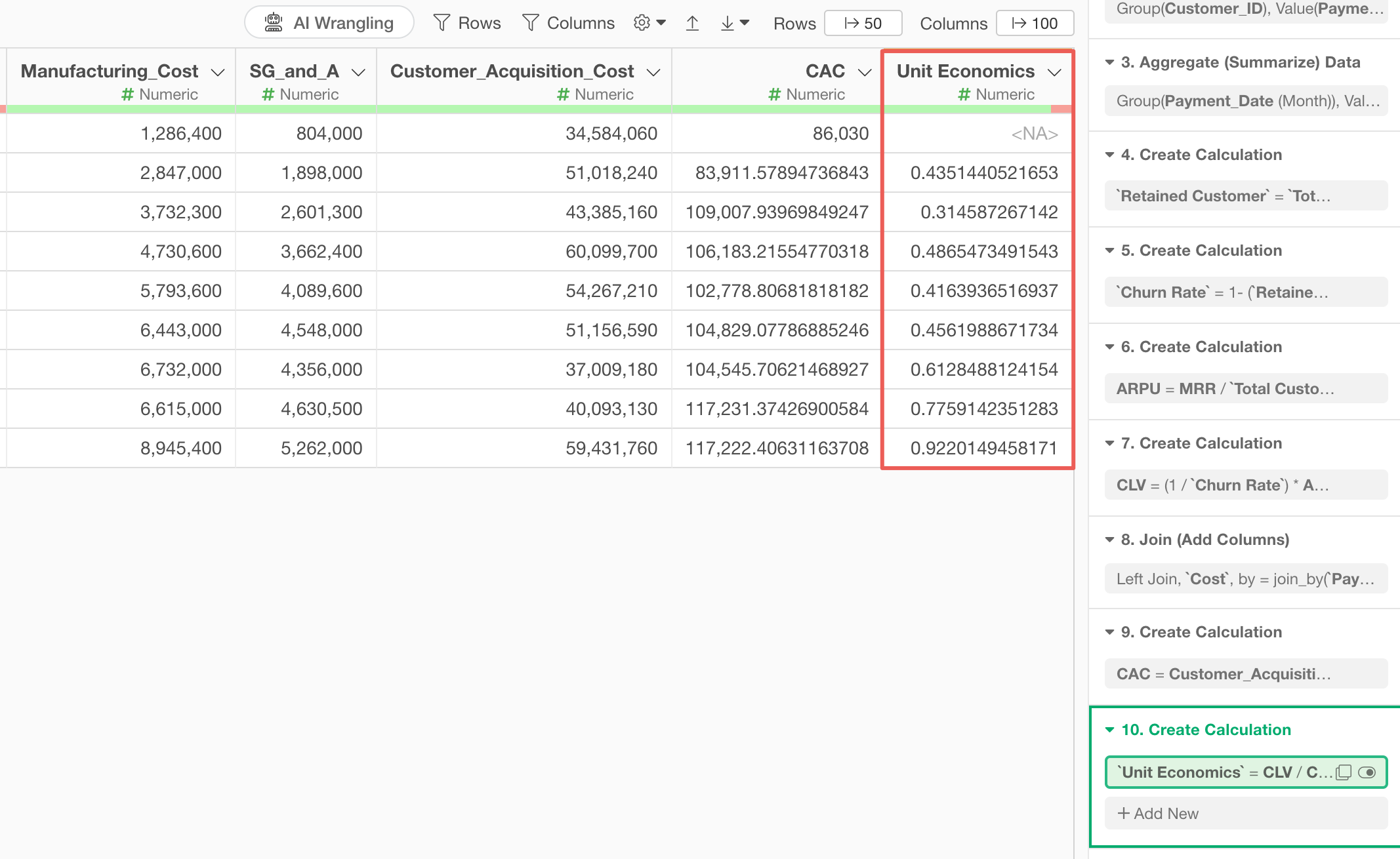
Now that we have both “CAC” and “CLV” needed for Unit Economics calculation, we will calculate “Unit Economics”.

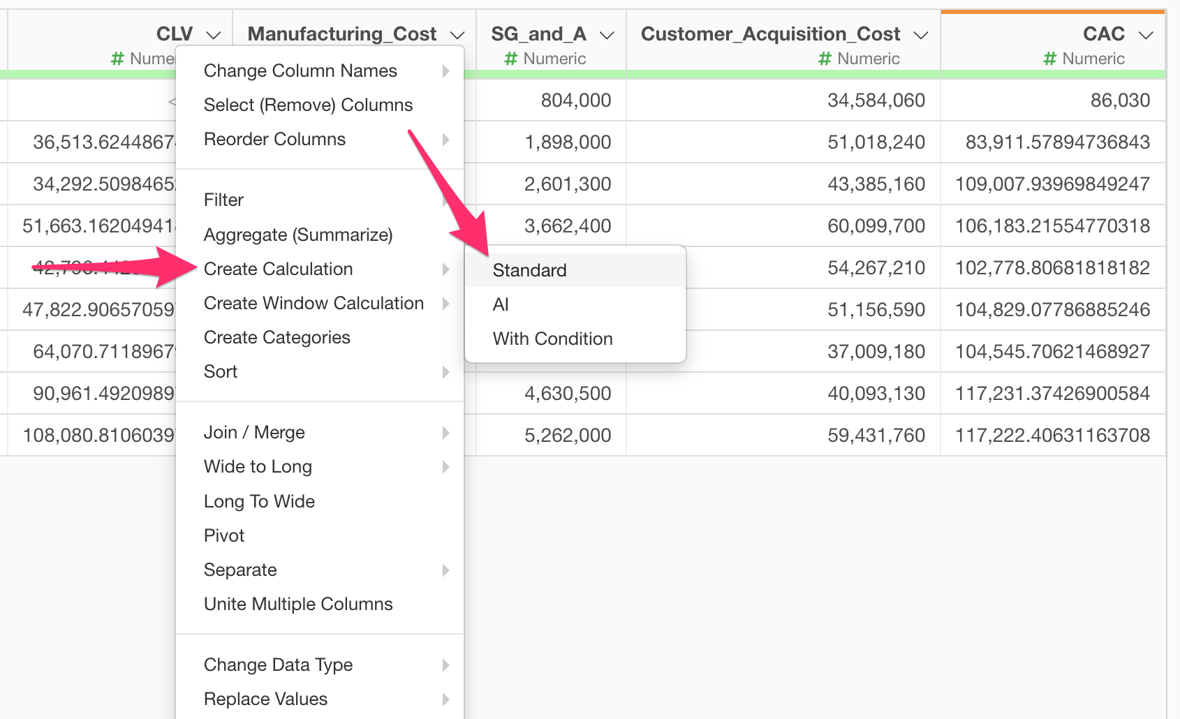
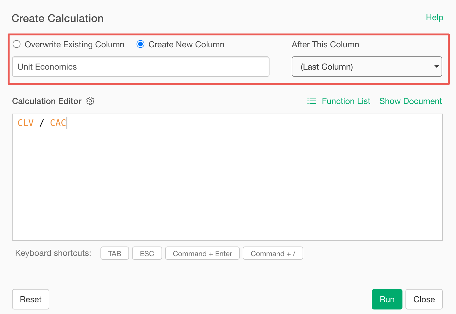
Select “Create Calculation” and “Standard” from the column header menu of CLV.

When the create calculation dialog opens, enter CLV / CAC in the calculation editor.

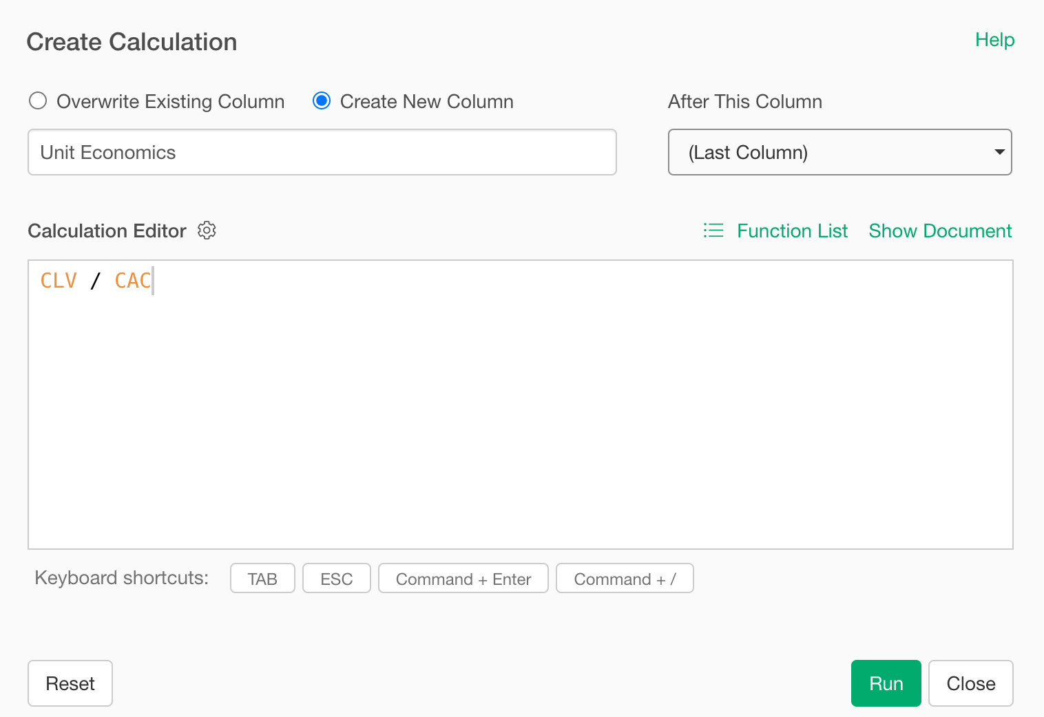
Finally, confirm that “Create New Column” is checked, set the column name to “Unit Economics”, change “After This Column” to the last column, and click the “Run” button.

We have successfully calculated Unit Economics.