Subscription Data Analysis #3 - Conversion Factor Analysis and Prediction

This note is the third installment of the “Subscription Data Analysis” trial tour, “Conversion Factor Analysis and Prediction,” which efficiently teaches you how to create, visualize, and analyze metrics specific to subscription-based businesses.

In subscription-based businesses, new customer conversion (acquisition) is essential for business growth.

And if you can identify customer segments and behaviors that are more likely to convert, you can use this information for customer targeting to increase the number of converting customers.

Furthermore, if you can predict the probability of conversion for each prospect, you can focus on supporting customers with a high probability of conversion to improve customer acquisition efficiency.

In this note, we will create a model to predict prospect conversion using “Random Forest,” one of the most frequently used machine learning algorithms by data scientists, and analyze the characteristics of customers who are likely to convert.

Additionally, we will use the created prediction model to predict the probability of conversion for prospects who are currently in the trial period.

It takes about 20 minutes. Let’s get started!!

What is a Prediction Model?

For example, let’s consider a video streaming service like Netflix.

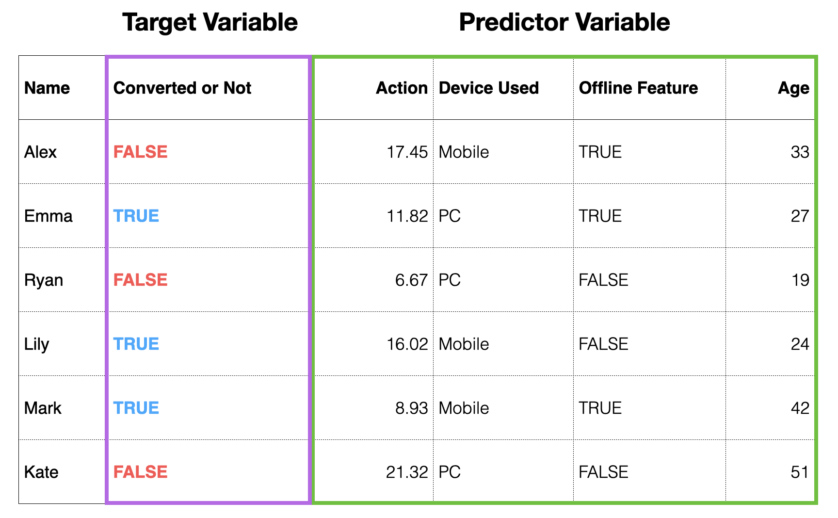
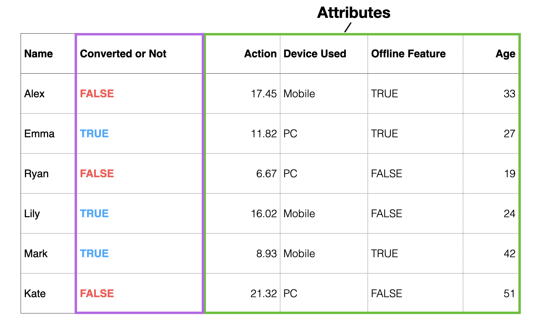
Suppose you have data as shown below, where each row represents one customer, showing who converted to a paid customer in the past, along with customer attribute information.

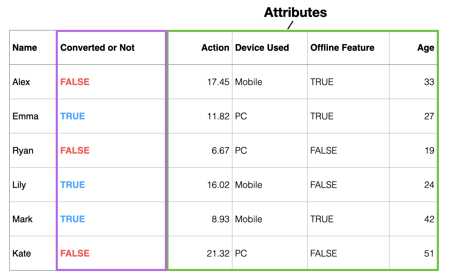
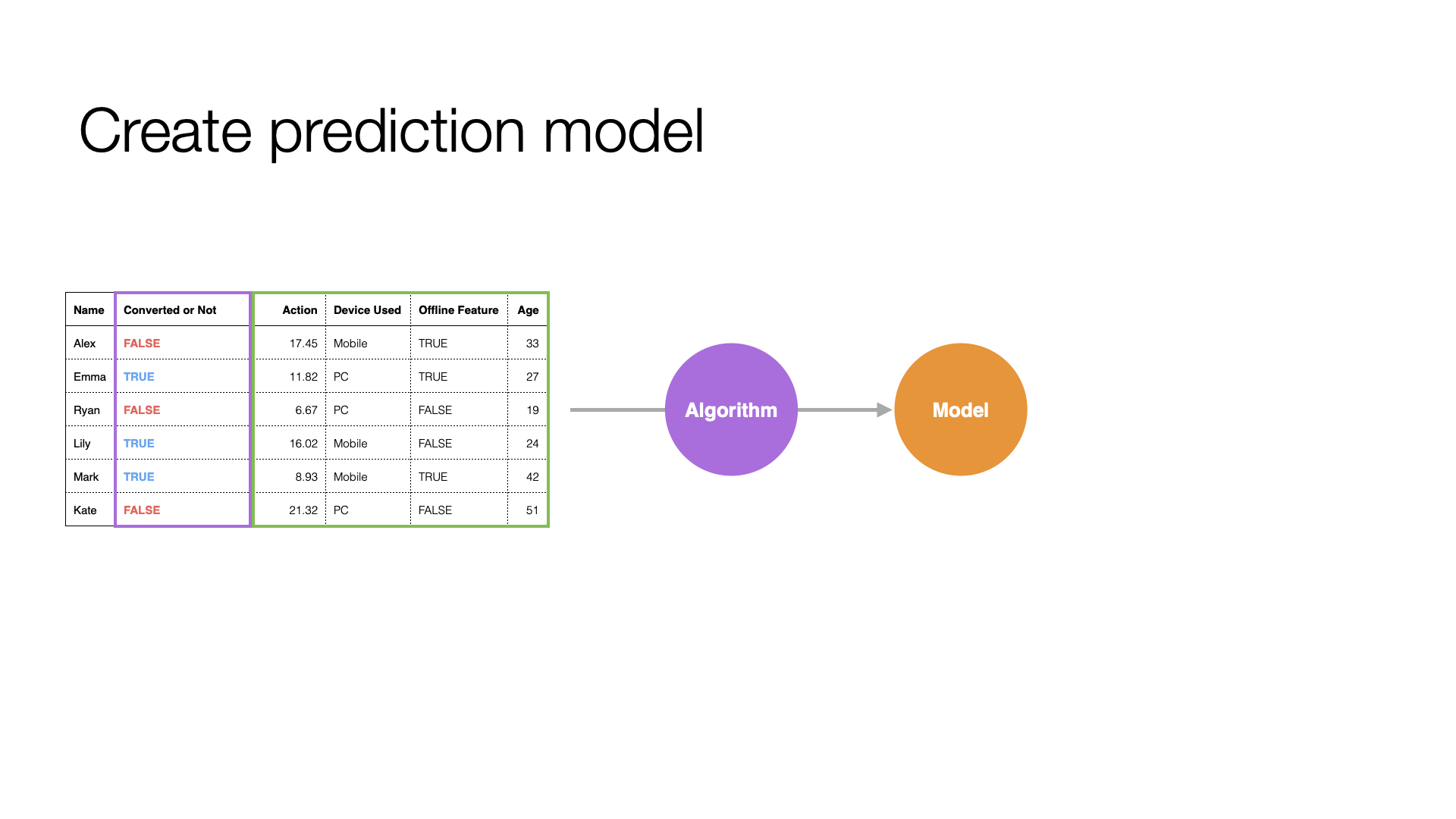
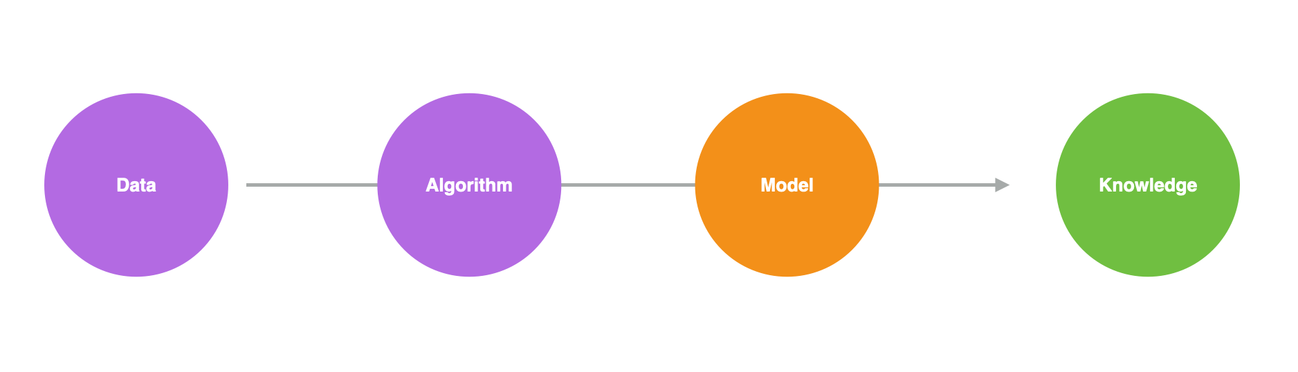
With such data, you can use statistical or machine learning “algorithms” to formulate or create rules based on the relationship between customer attributes and conversion to predict future behavior by identifying patterns in historical data.

This expression of patterns detected by algorithms in the data is called a “prediction model.”

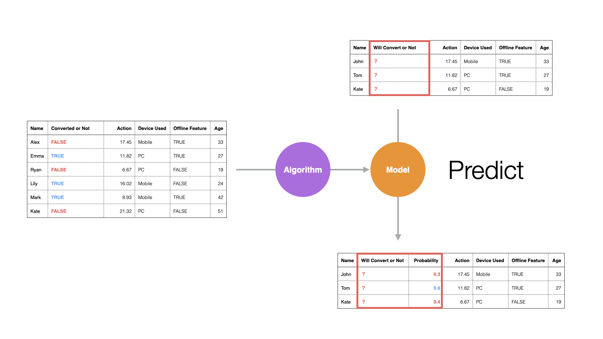
Using a prediction model, you can predict who among new prospects will convert.

In the world of data science, the target to predict (“whether converted or not”) is called the “objective variable,” and the information used for prediction is called the “predictor variable” or “explanatory variable.”

Also, creating a prediction model helps you understand patterns in the data, such as:

Which variables have a strong relationship with the objective variable (conversion)
What kind of relationship it is
Whether the relationship is significant
How much of the objective variable’s movement can be explained by this model

Data Overview

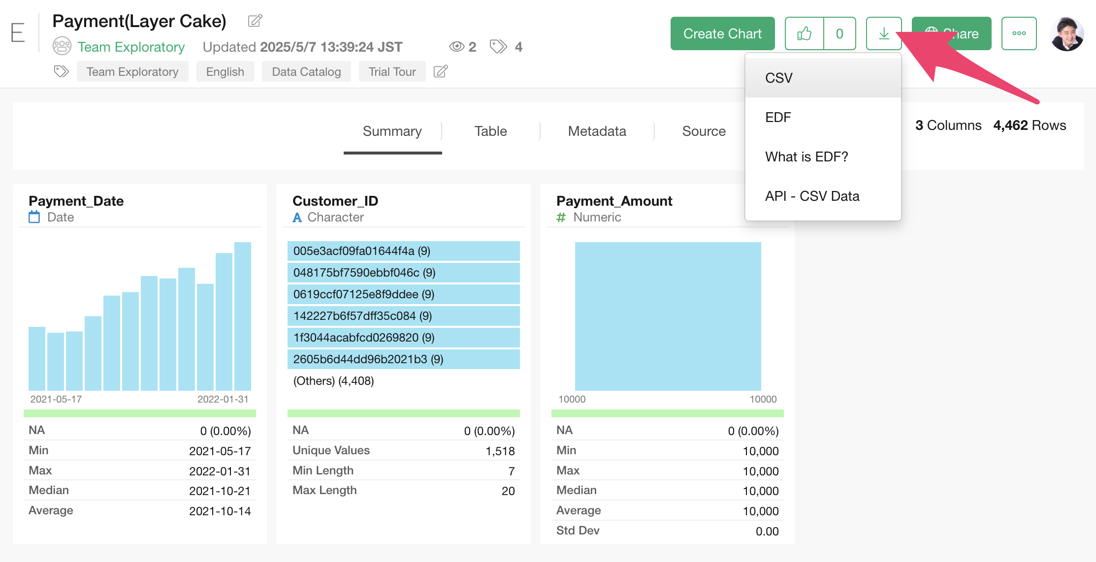
The sample data for this exercise is from a video streaming service like Netflix, showing service usage during the trial period. The data can be downloaded from this page.

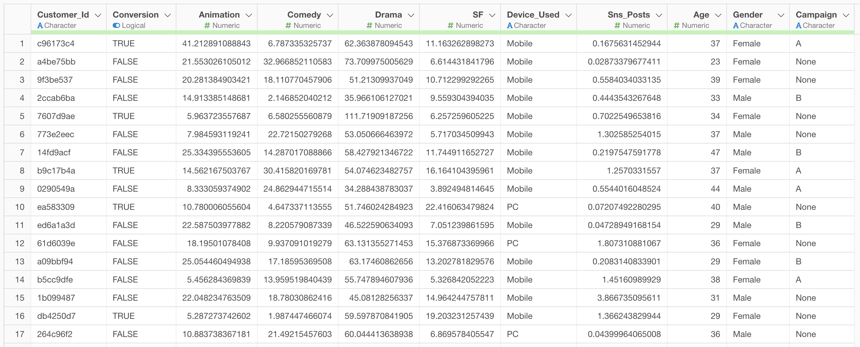
In this data, each row represents one prospect who signed up for a trial, and the columns contain the following information:

Whether they converted or not
Viewing time for each content type
Main device used
Age
Gender
Campaign that led to sign-up

Importing Data

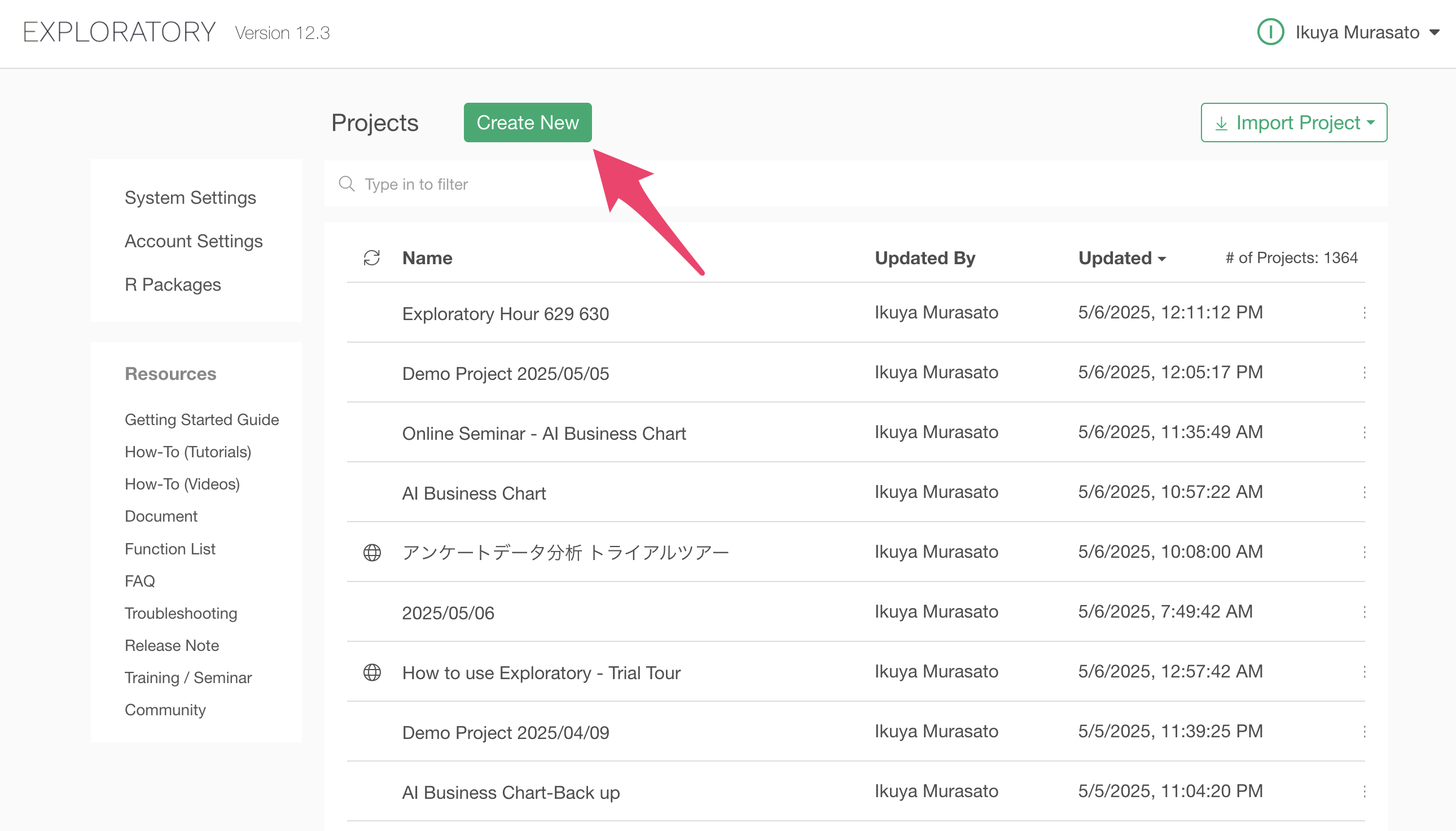
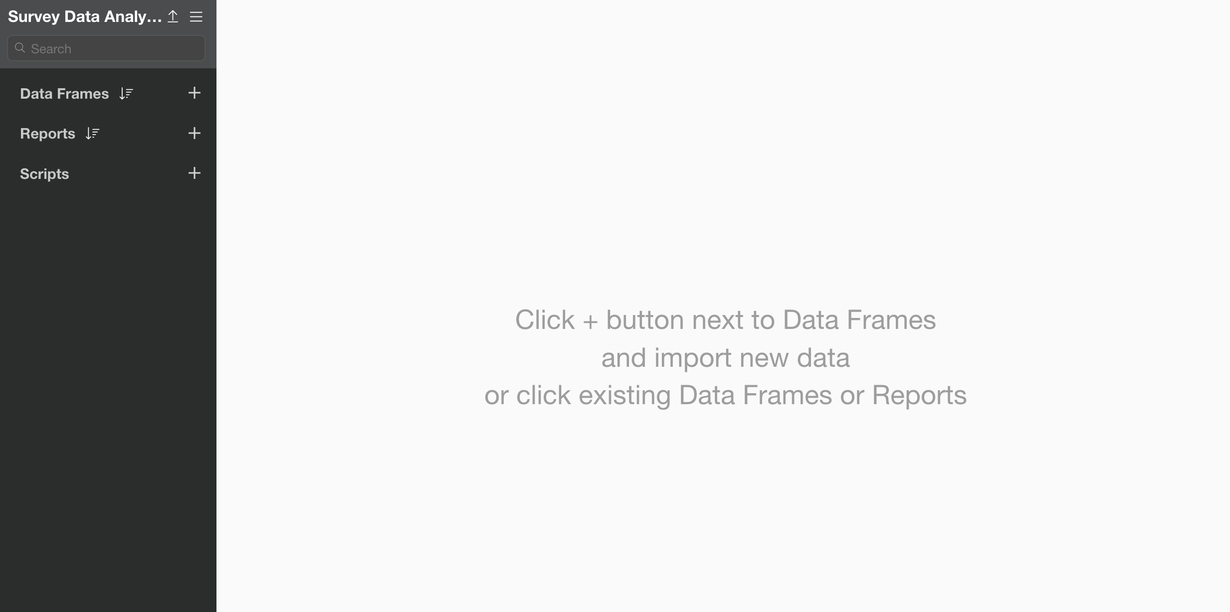
After launching Exploratory, click the “Create New” project button.

A dialog to create a project will appear. Enter any name you like and click the create button.

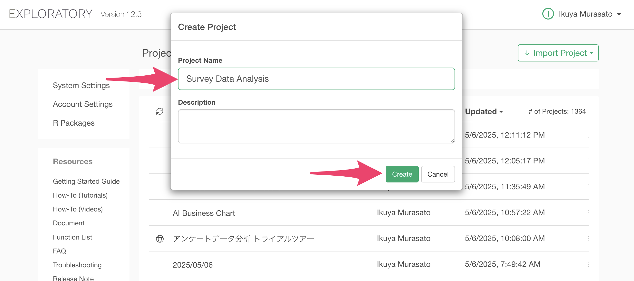
The project has been created.

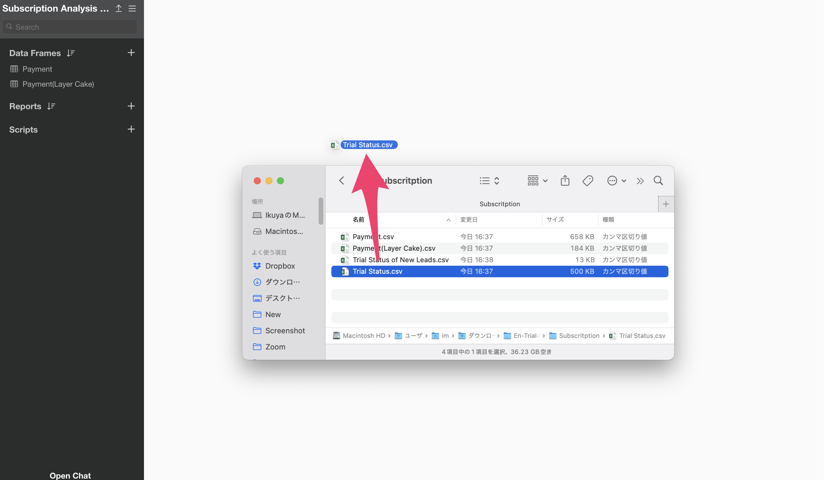
After creating the project, let’s import the data. The data can be downloaded from this page.

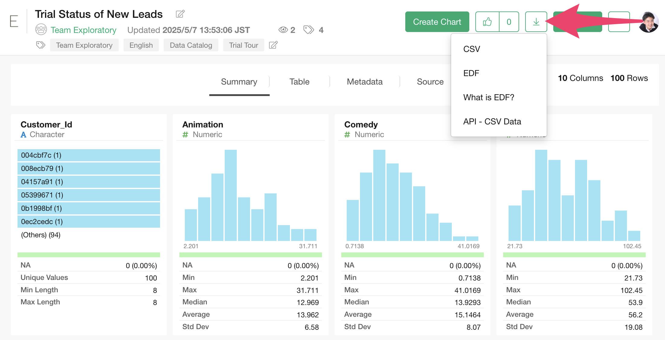
After downloading the customer trial status data, open the downloaded folder and drag and drop it onto the Exploratory screen.

An import dialog will appear.

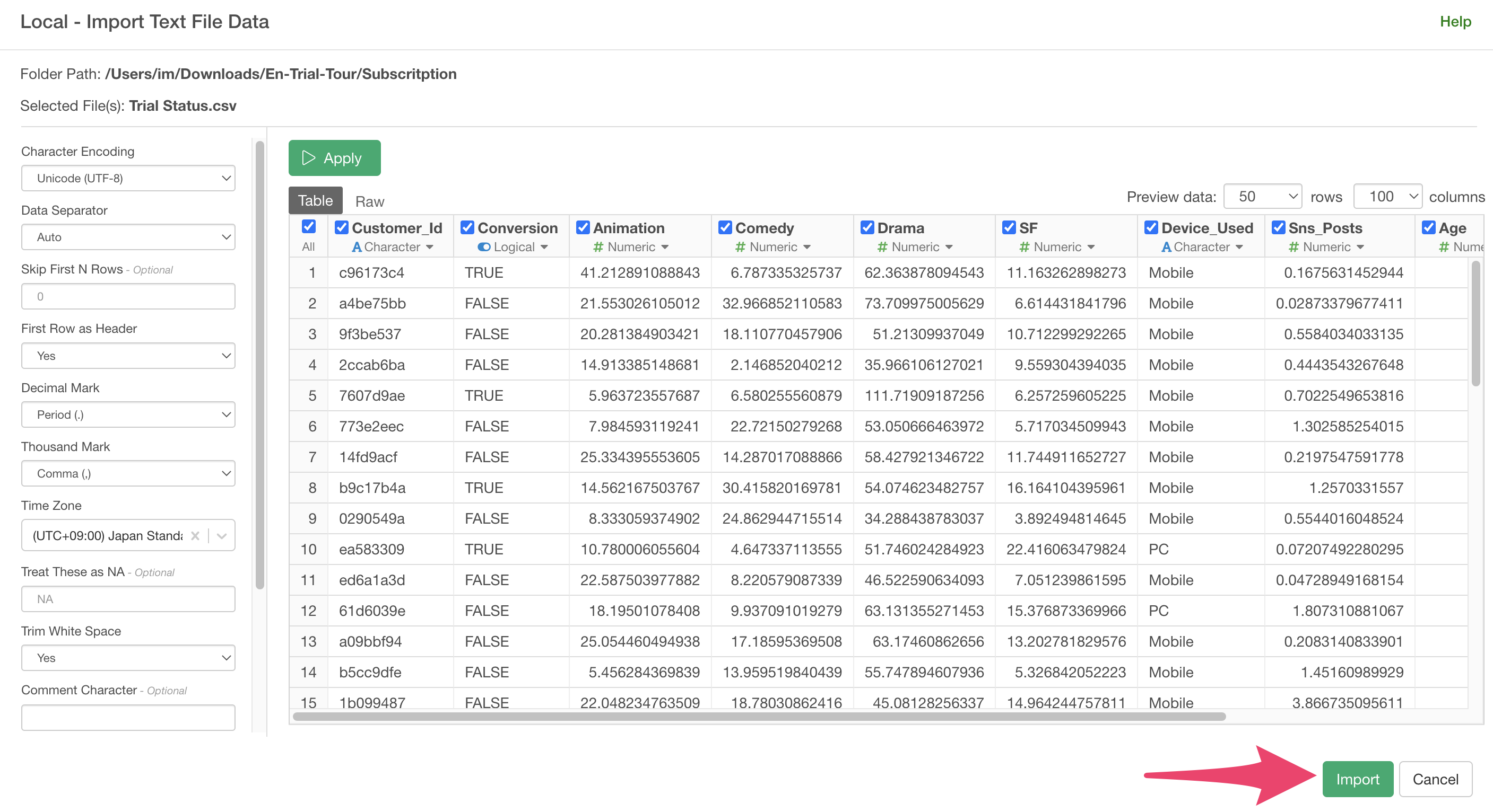
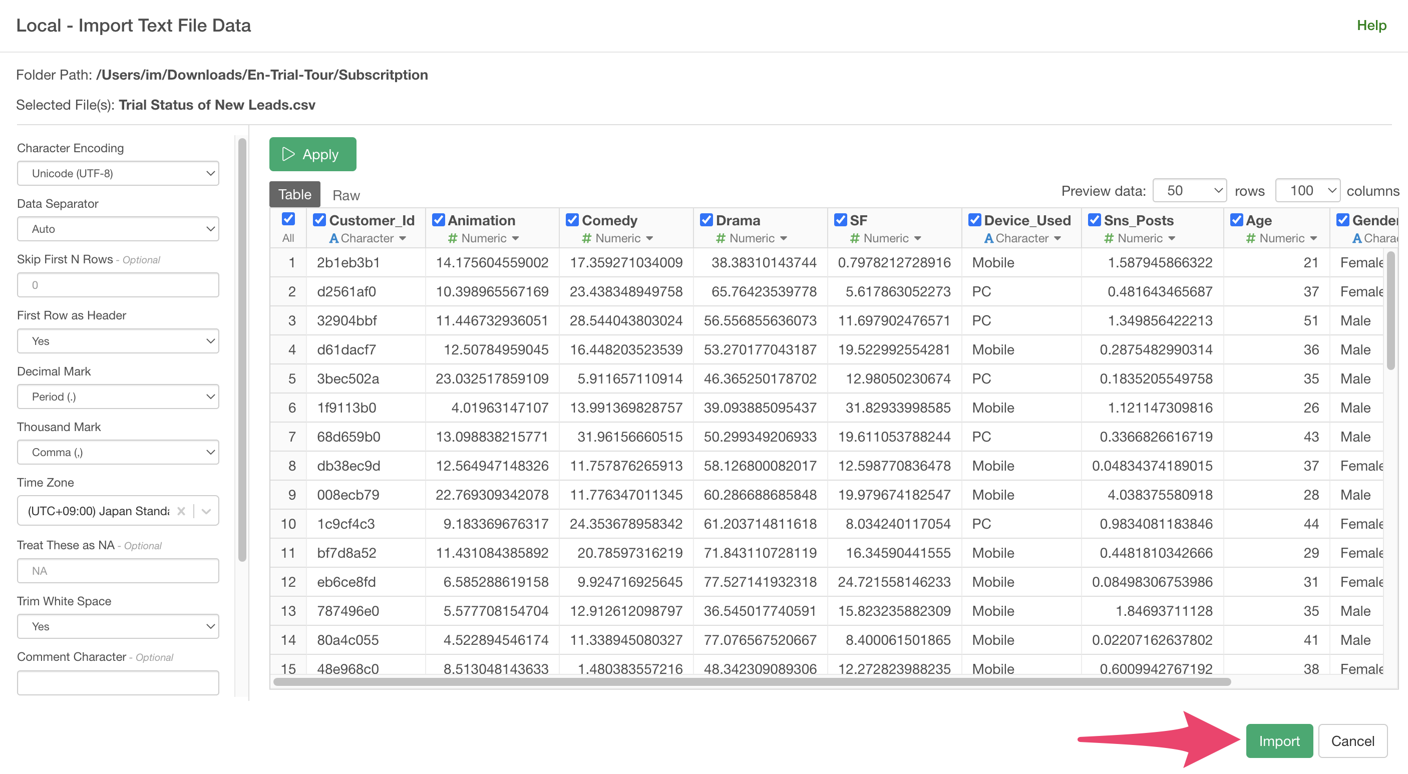
In the import dialog, you can specify settings for importing data from the items on the left, but no settings are needed this time, so click the “Import” button.

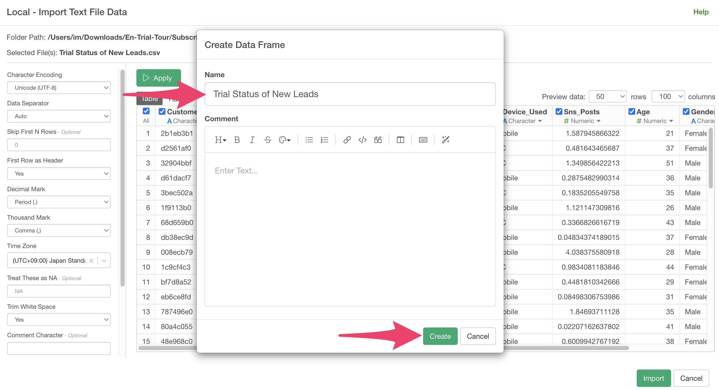
A data frame settings dialog will appear, so click the “Create” button.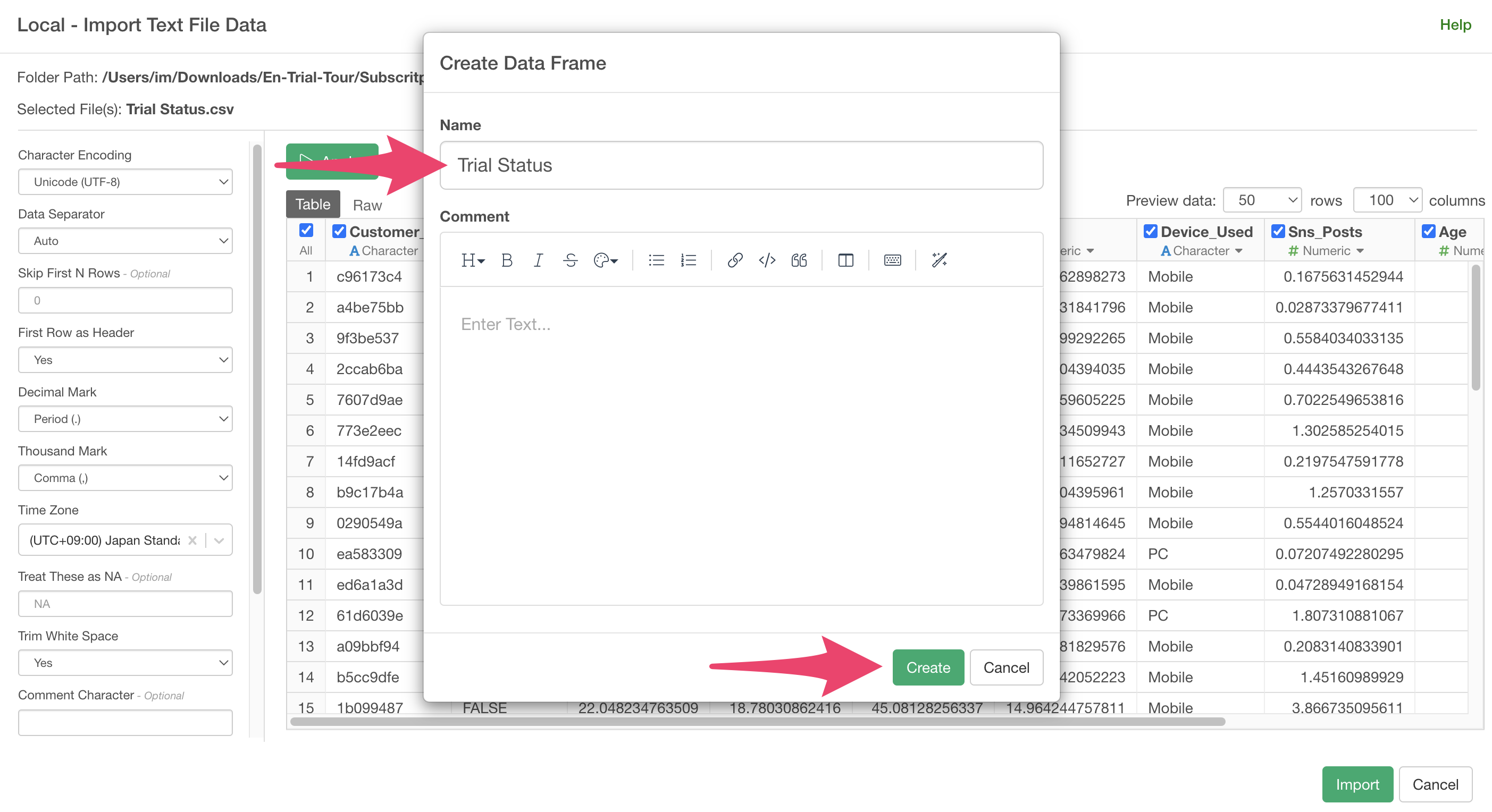

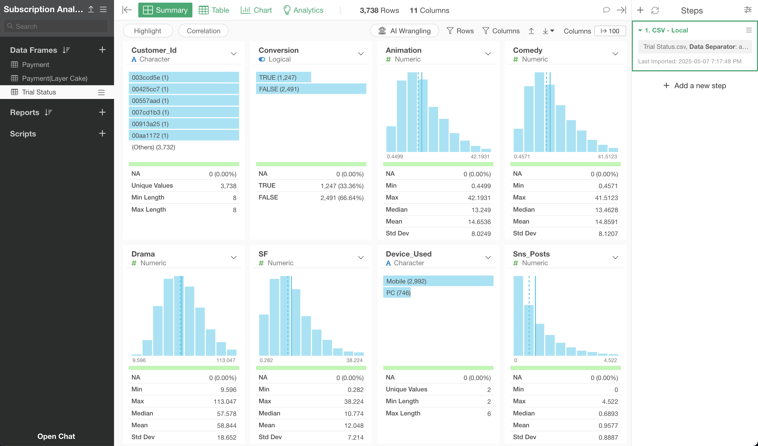
The customer trial status data has been imported.

Creating a Model to Predict Conversion Using Random Forest

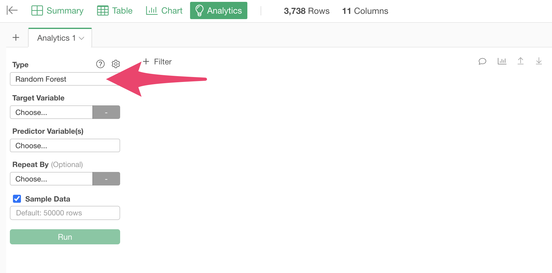
When you want to create a prediction model, move to the “Analytics View.”

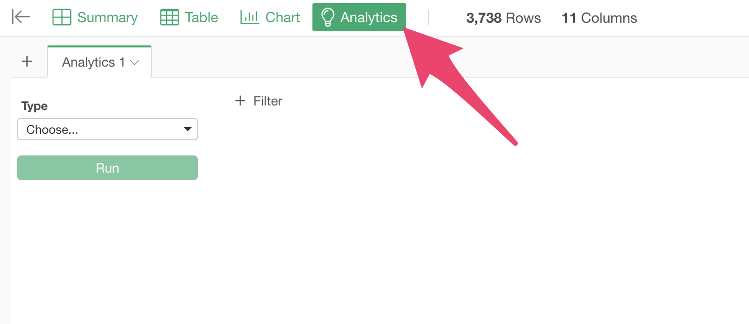
This time, we want to create a model to predict prospect conversion using “Random Forest,” one of the most frequently used machine learning algorithms by data scientists, so select “Random Forest” as the type.

For details on how to use Random Forest, please refer to this note.

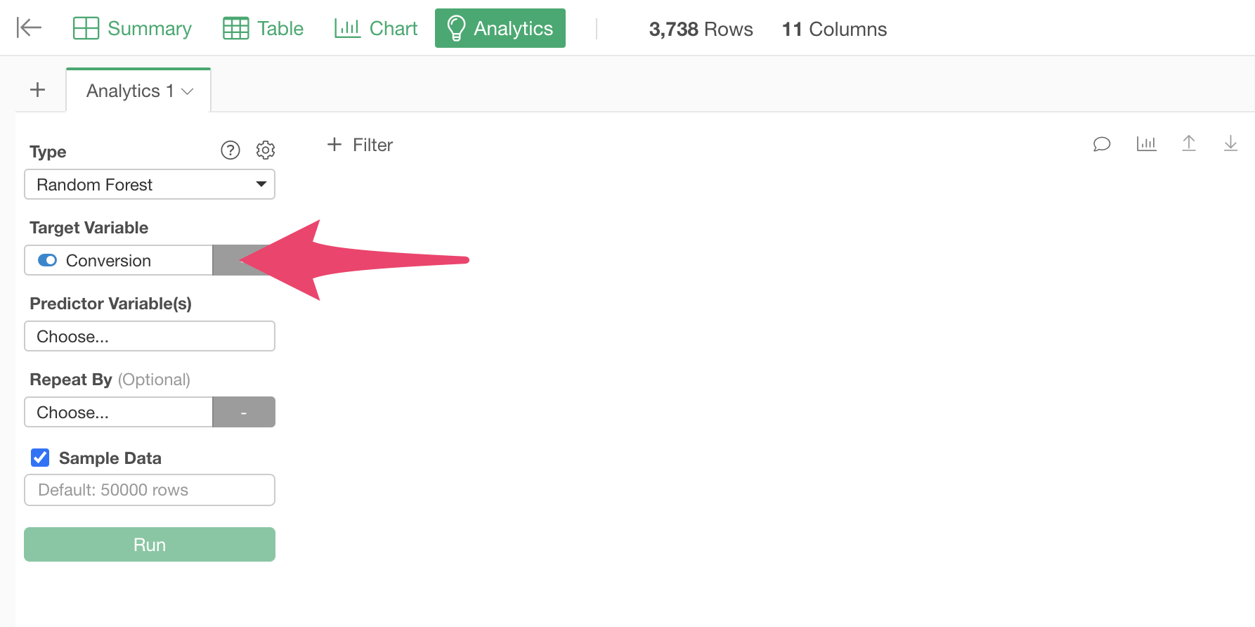
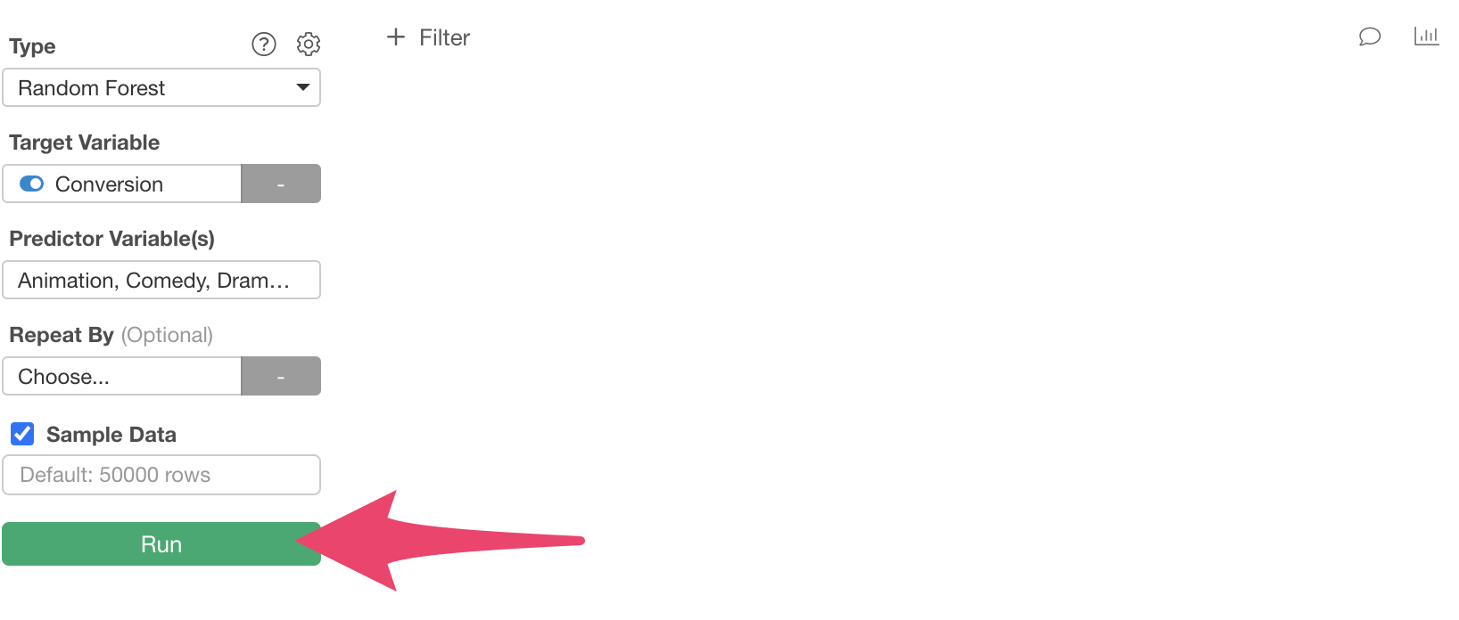
Next, select “Conversion” as the “Target Variable,” which is the column to be predicted.

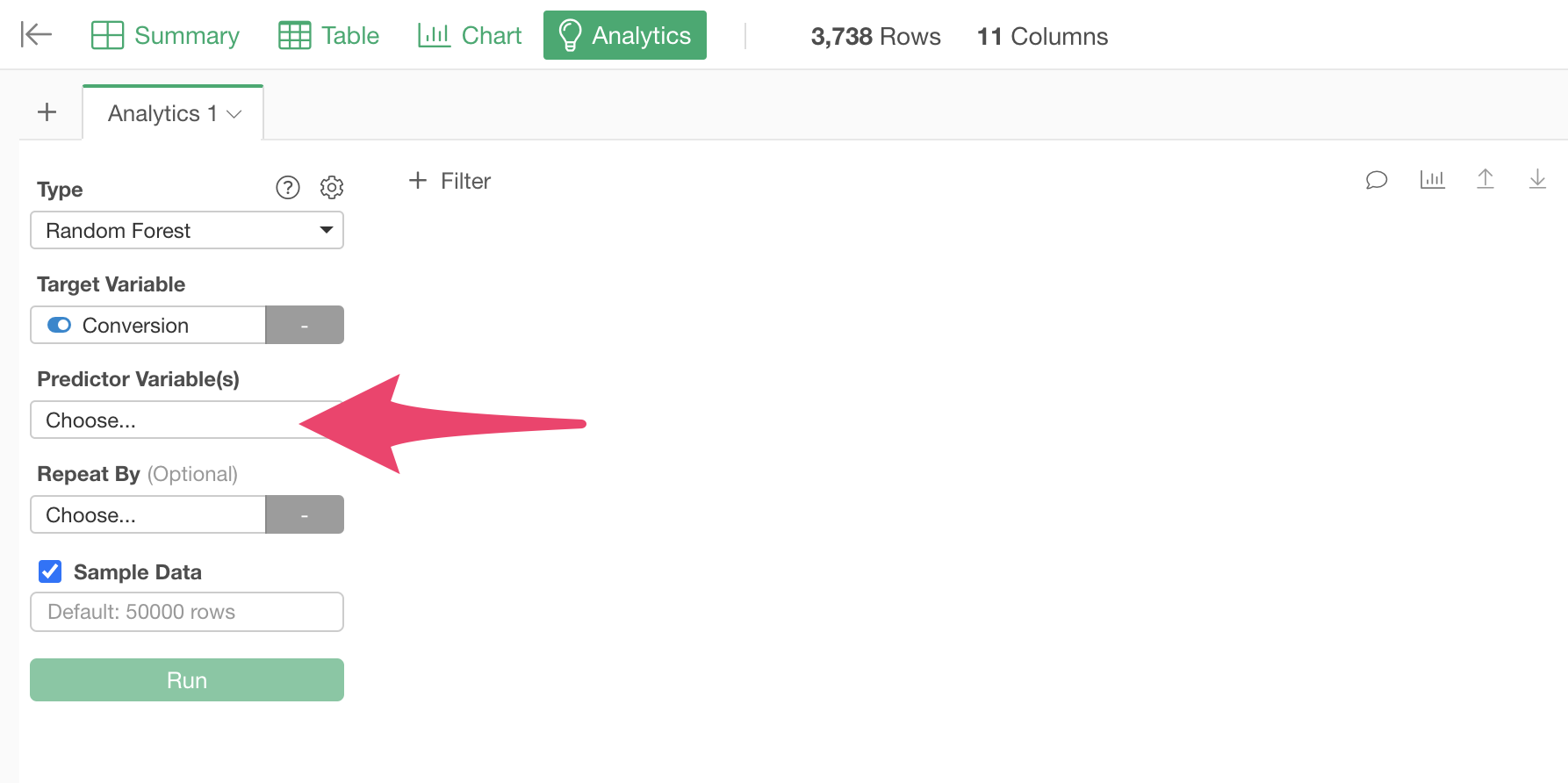
Next, select the predictor variables.

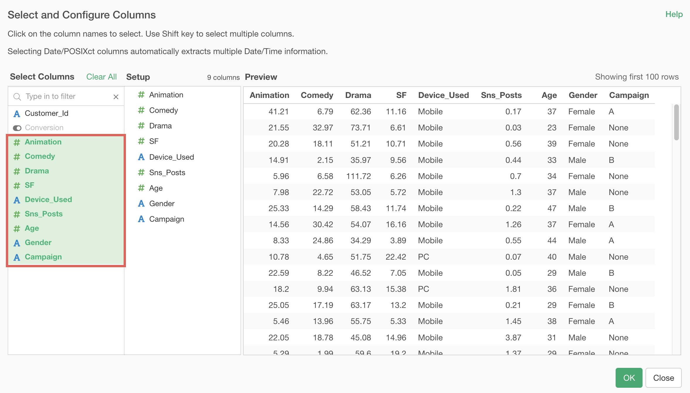
When the predictor variable selection dialog appears, hold down the Shift key and click on “Aniomation” and “Campaign” to select all columns except “Customer_ID,” then click the “OK” button.

Click the “Run” button.

A model to predict conversion has been created.

Interpreting the Prediction Model

When you run a prediction model, multiple tabs for interpreting the prediction model are displayed.

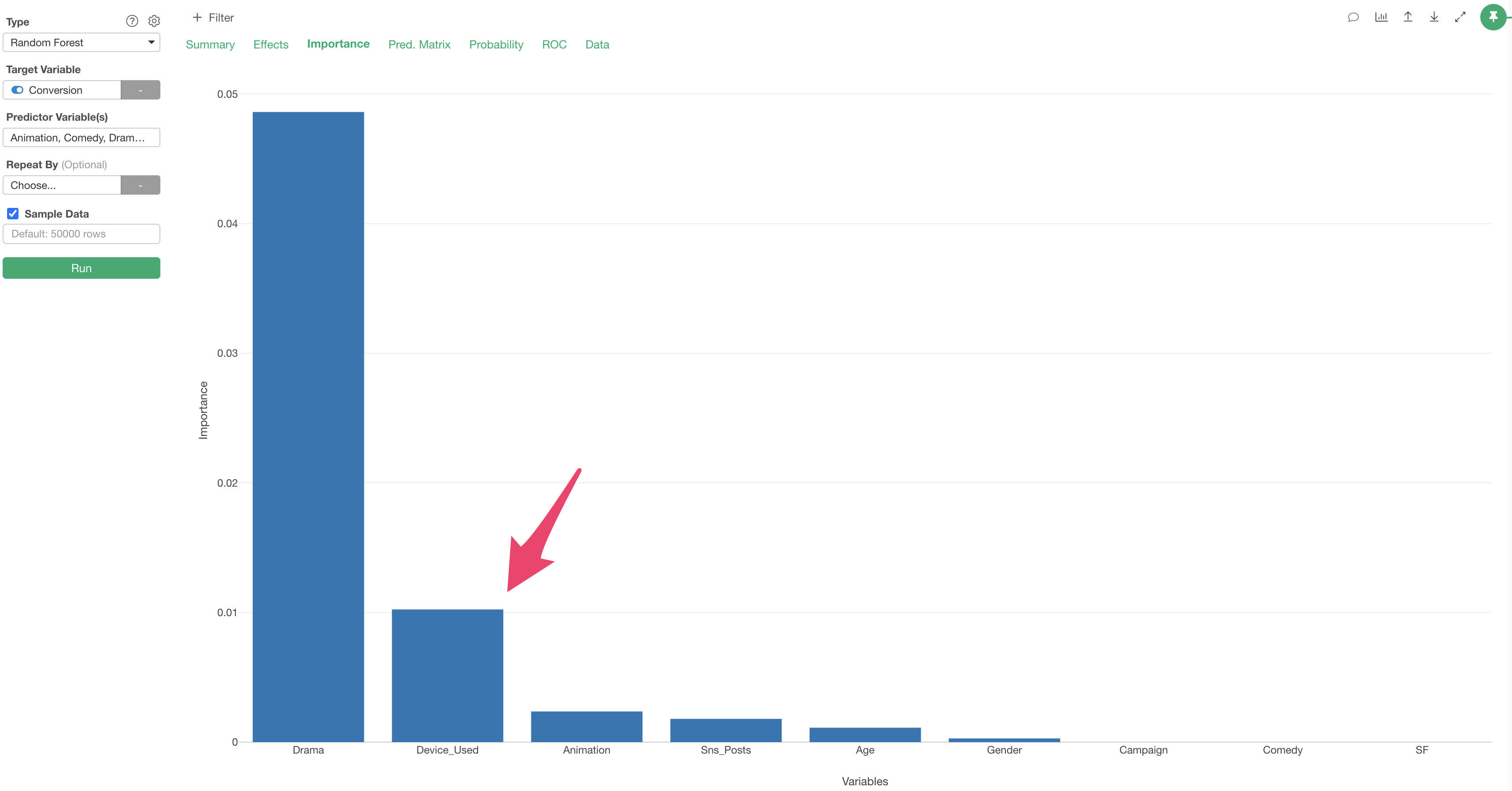
Variable Importance

In the Variable Importance tab, you can examine which variables have a stronger correlation with the objective variable (conversion) and which are more important for prediction.

The higher the bar, the stronger the correlation with the objective variable.

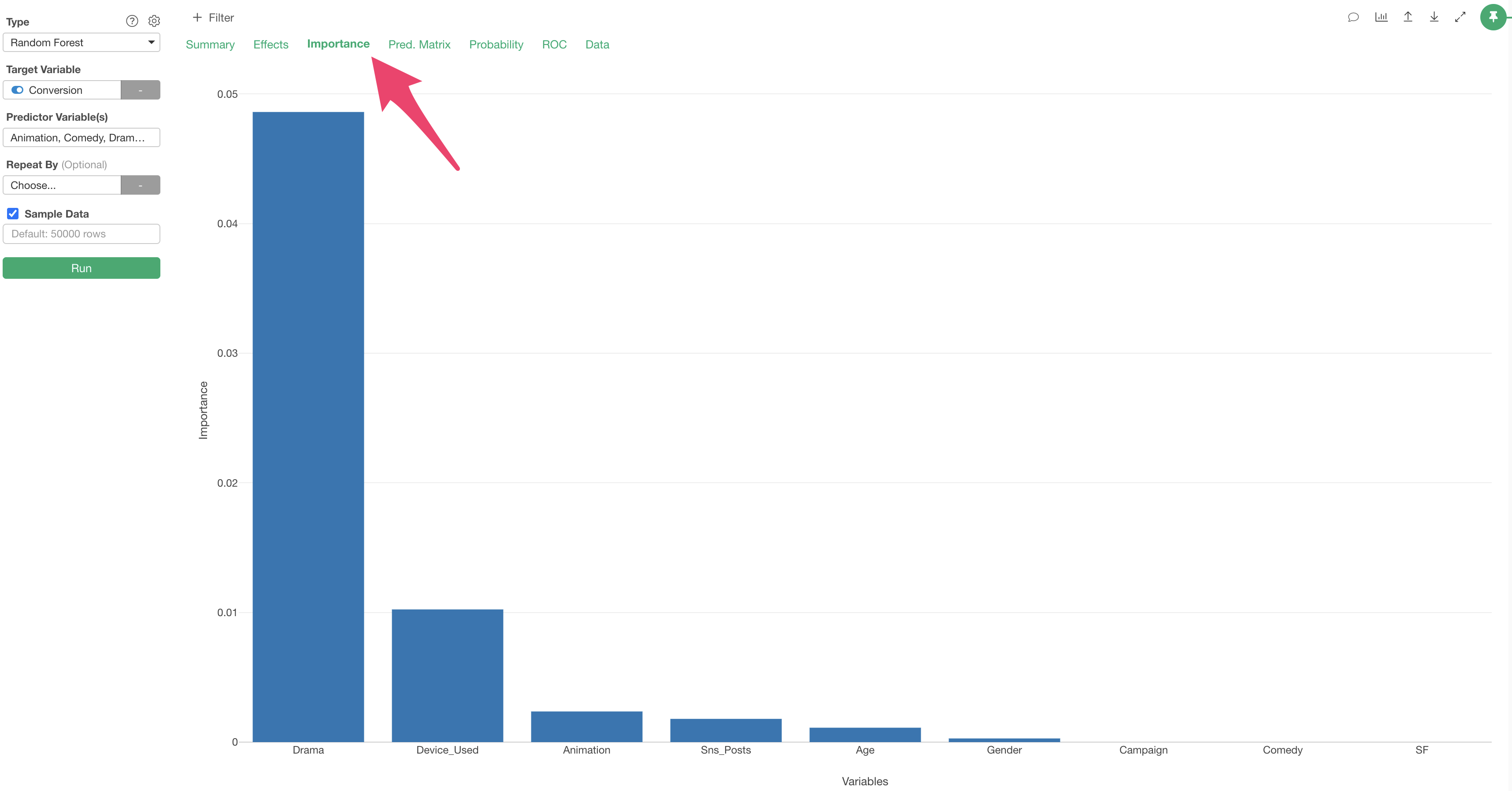
In this data, it appears that “Drama”viewing time is the most important variable for predicting conversion.

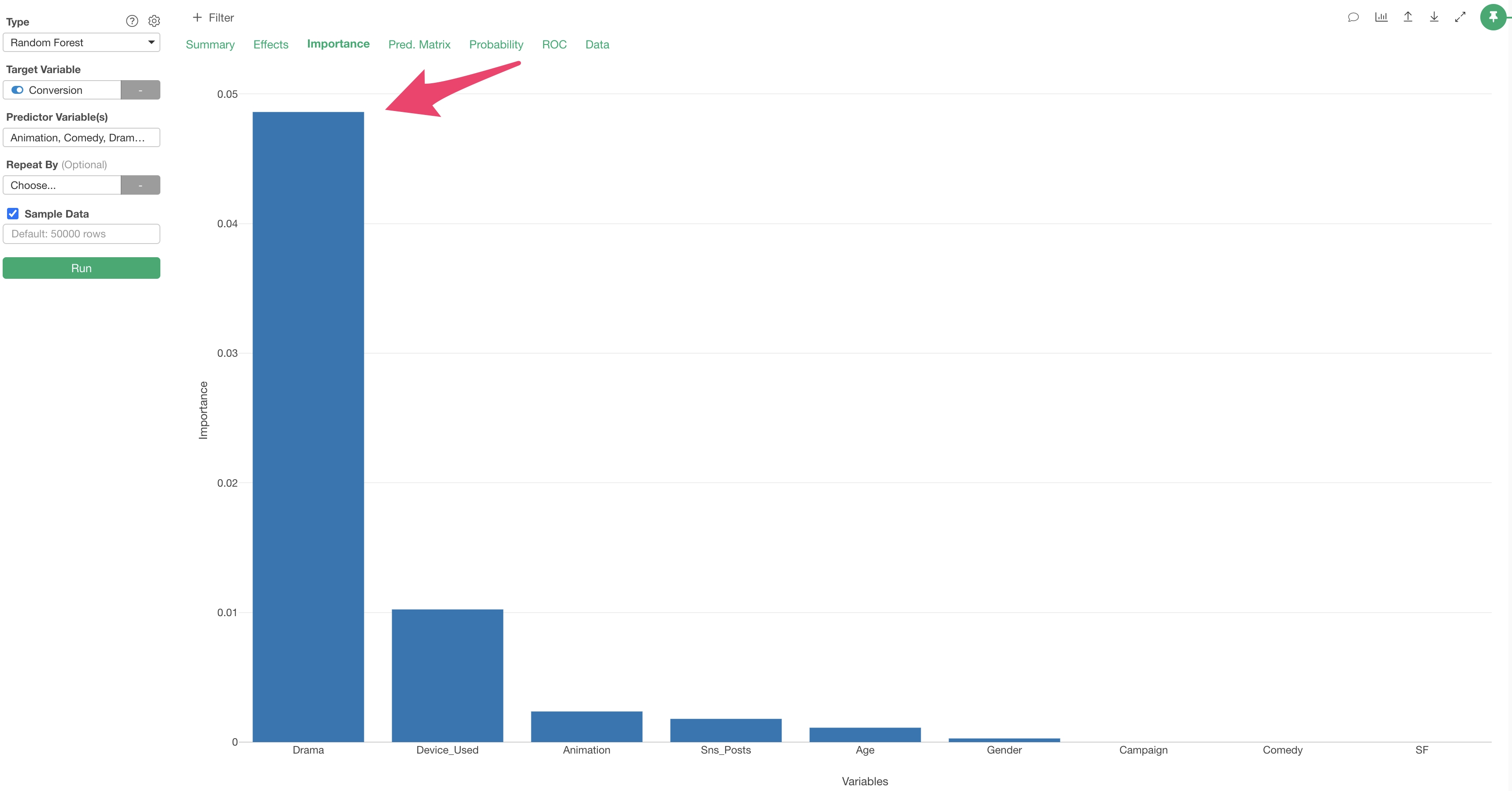
We can also see that “Device_Used” are important for predicting conversion too.

For more details on variable importance, please refer to this note.

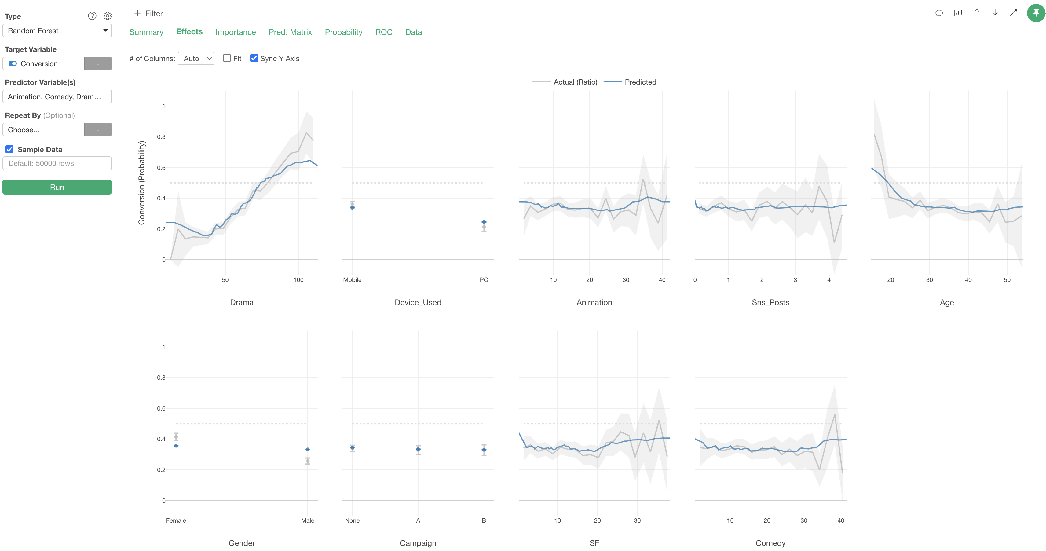
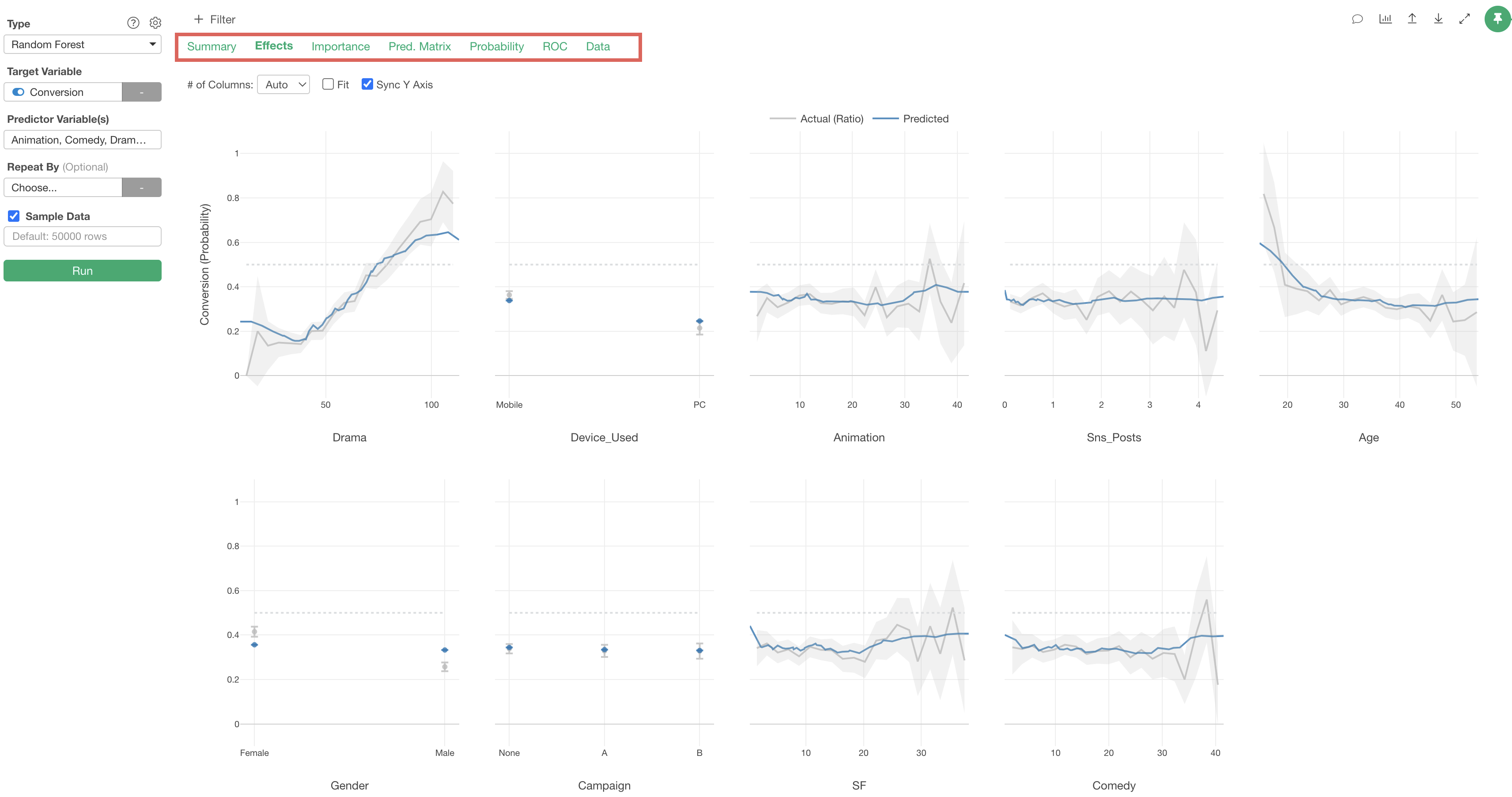
Effects

In the Effects tab, you can see how the value of the objective variable changes as the value of each variable changes.

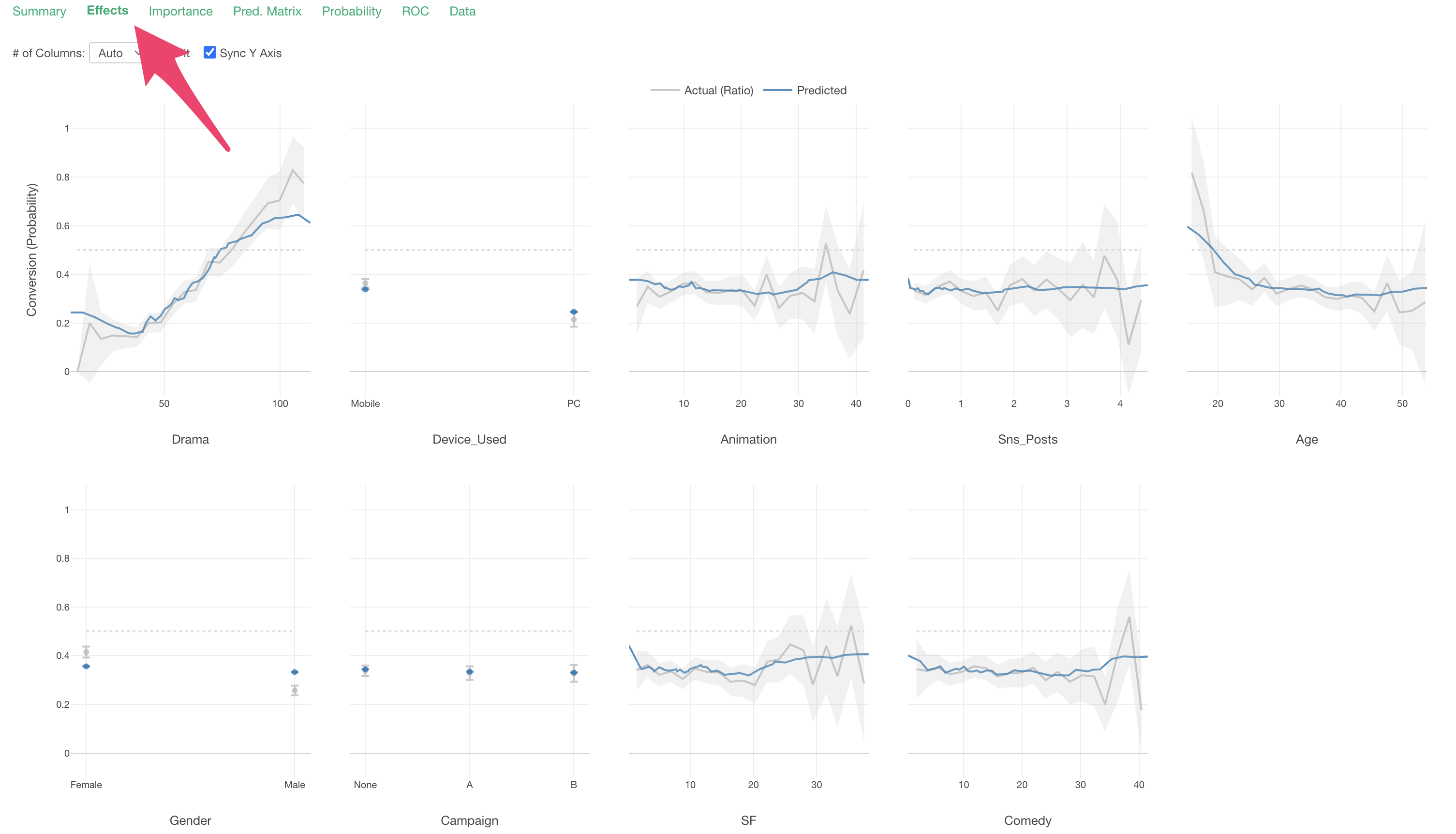
The X-axis represents the values of each “predictor variable,” and the Y-axis represents the proportion of TRUE for the variable selected as the “target variable” (conversion), so in this data, it represents the “conversion rate”.

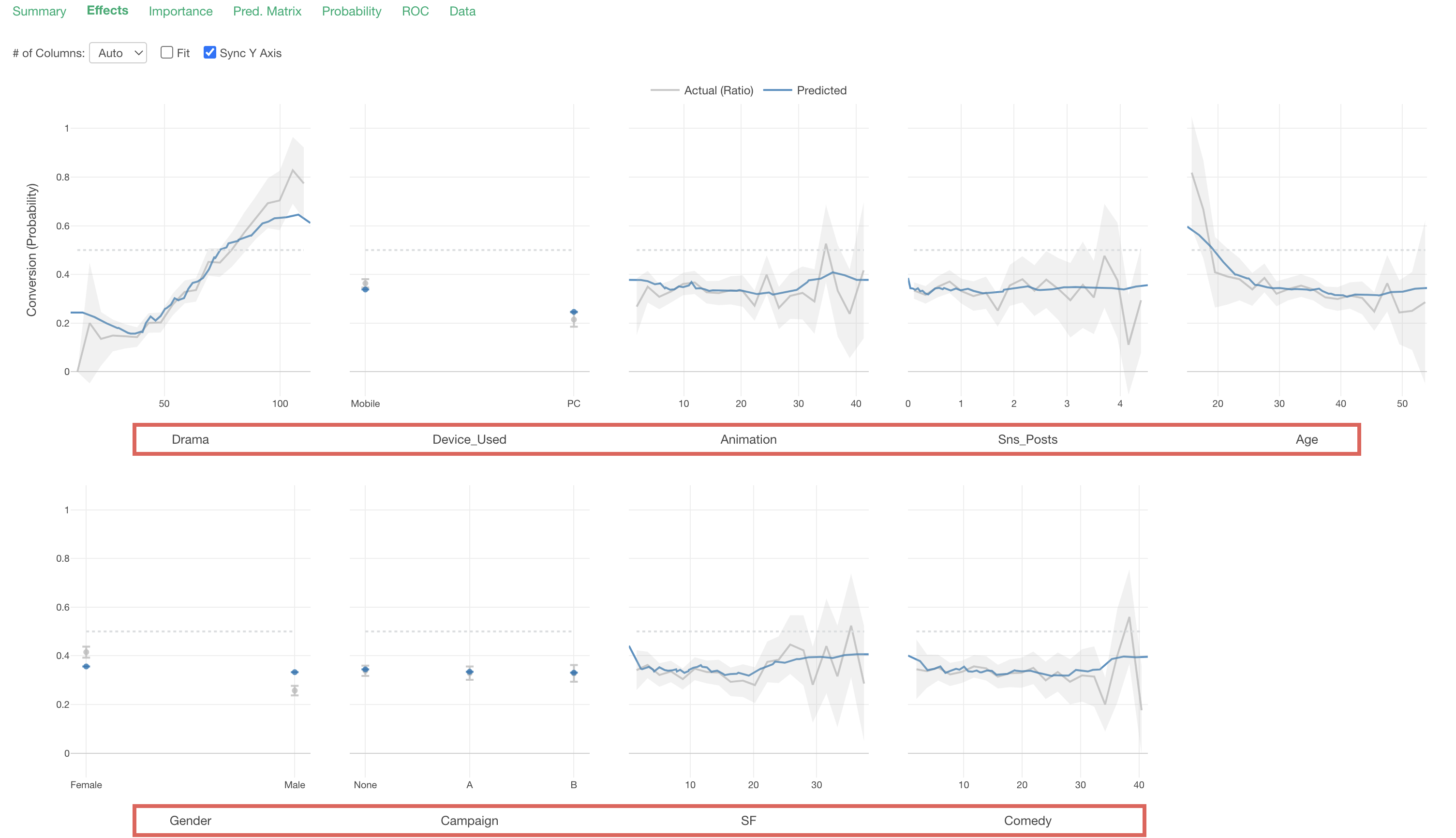
Each predictor variable is arranged in order of variable importance.

The gray line represents the measured values.

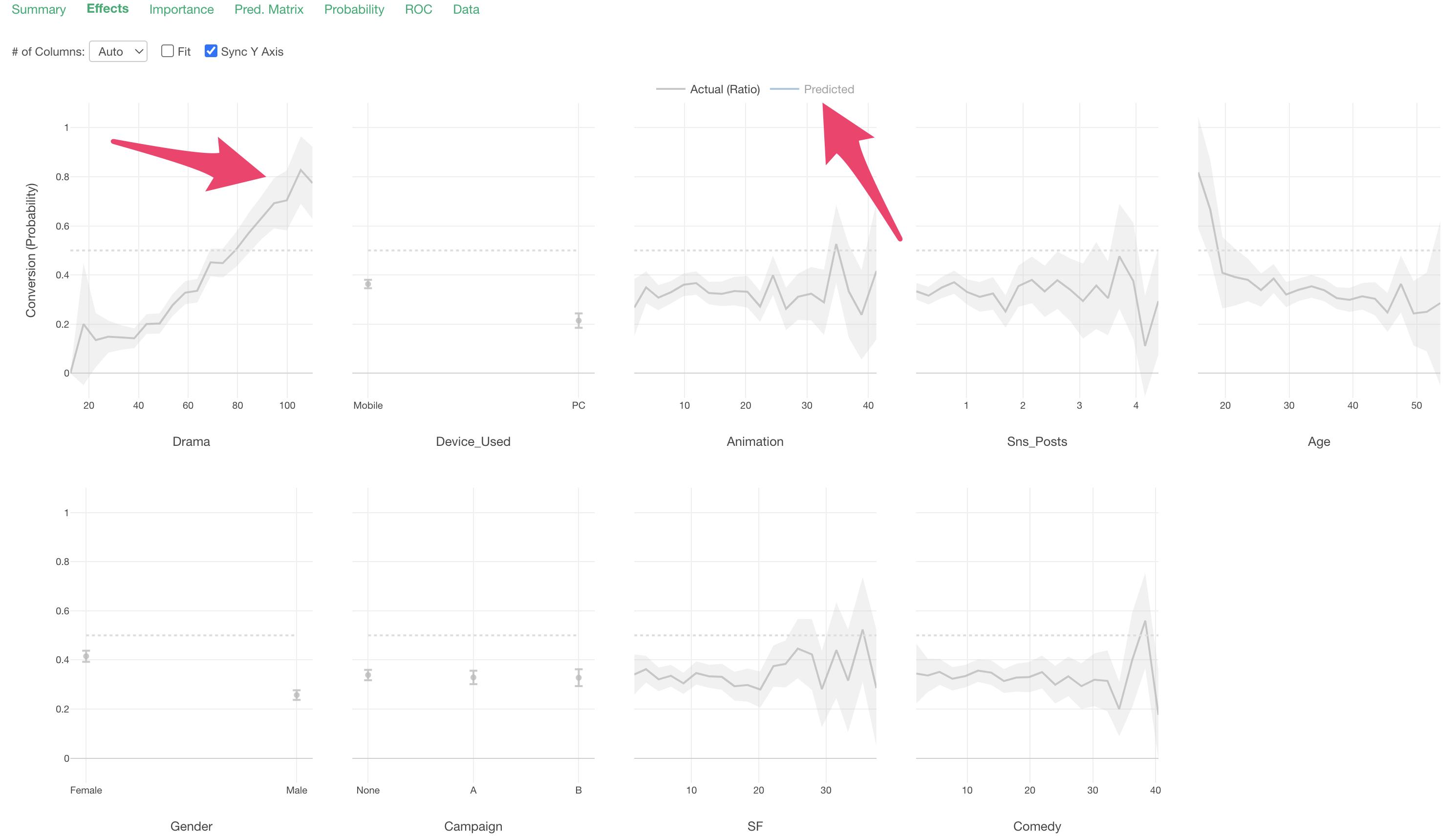
The blue line represents the predicted values.

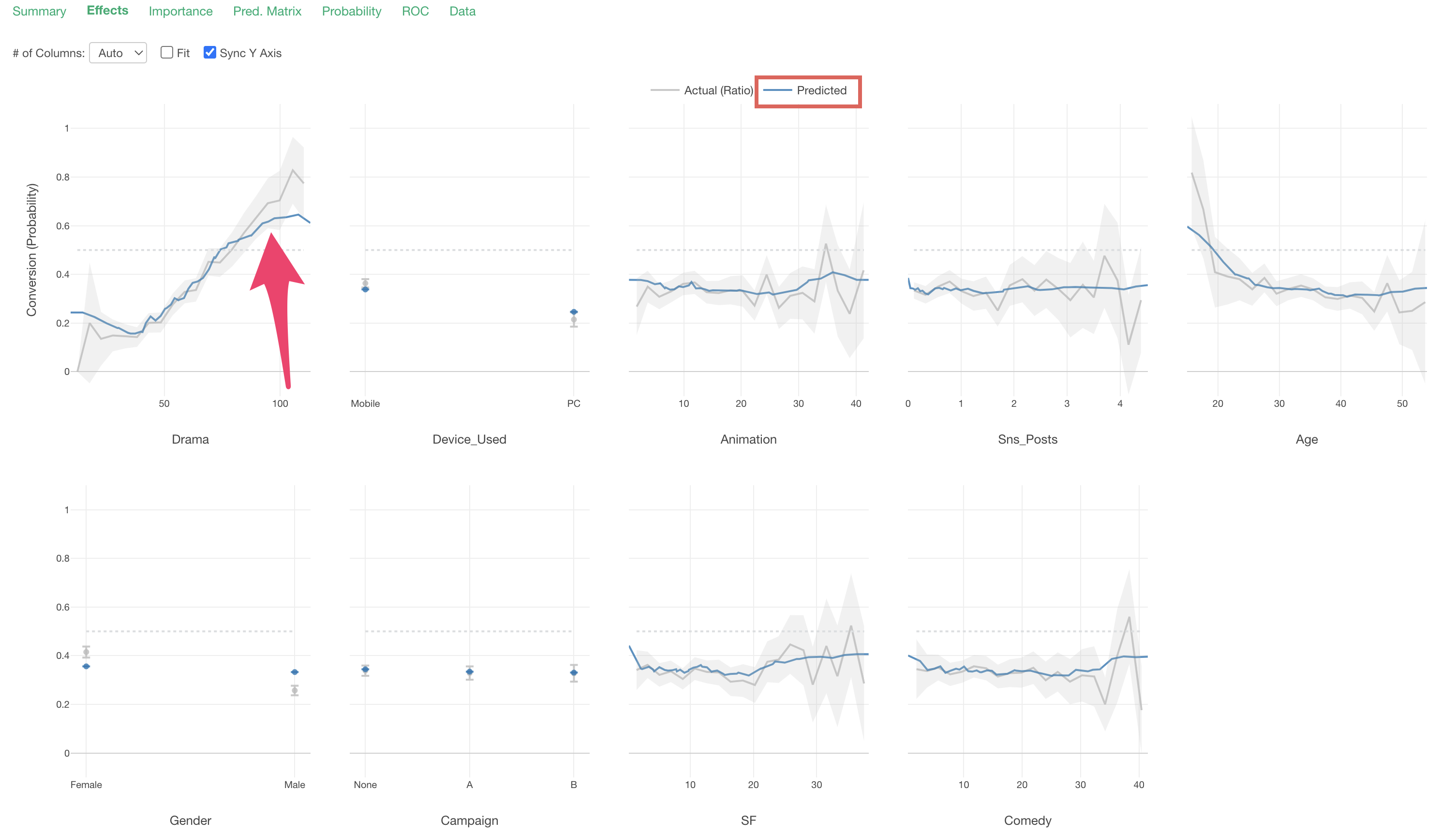
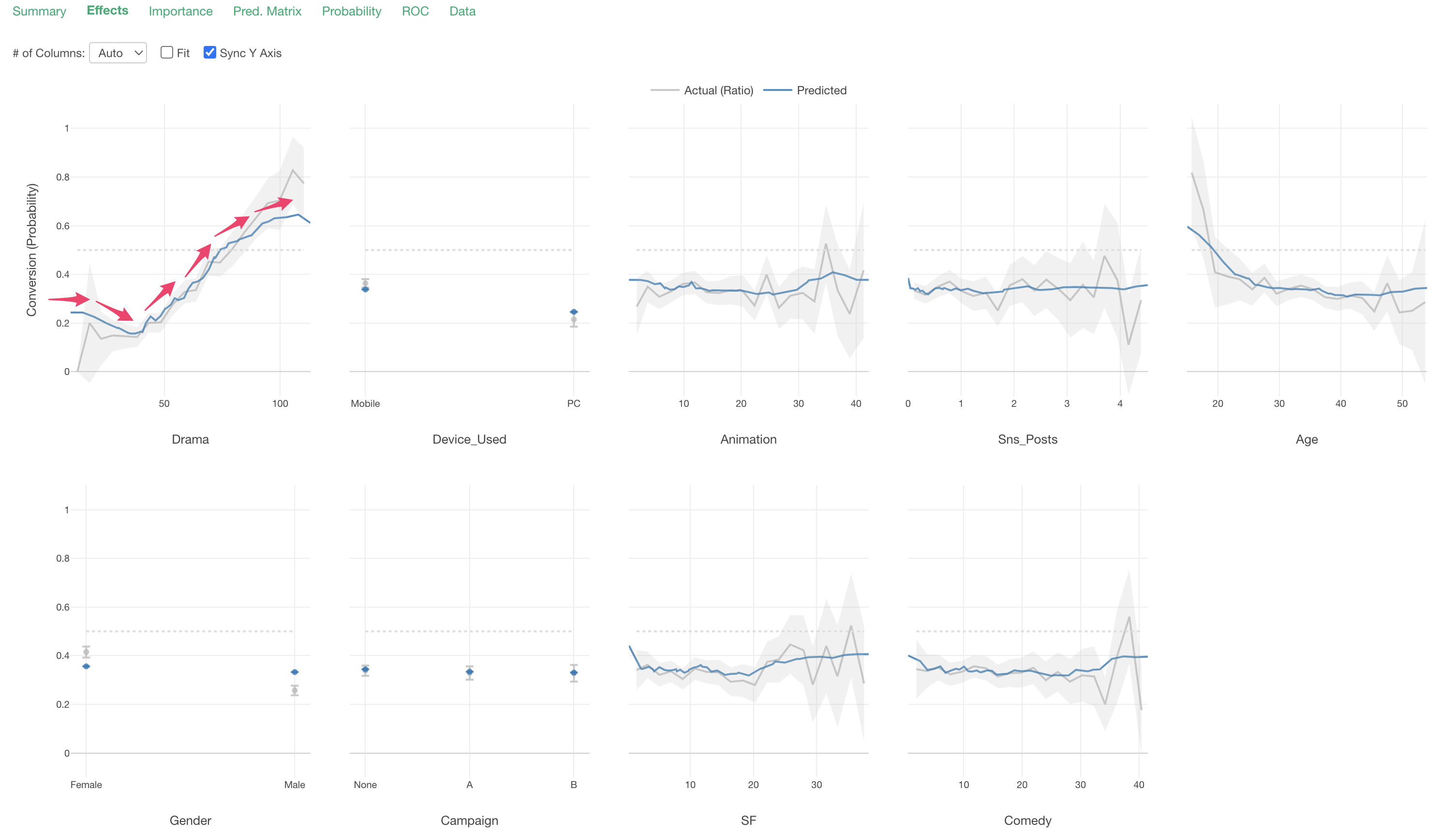
Looking at “Drama”, we can see that the conversion rate increases as viewing time increases.

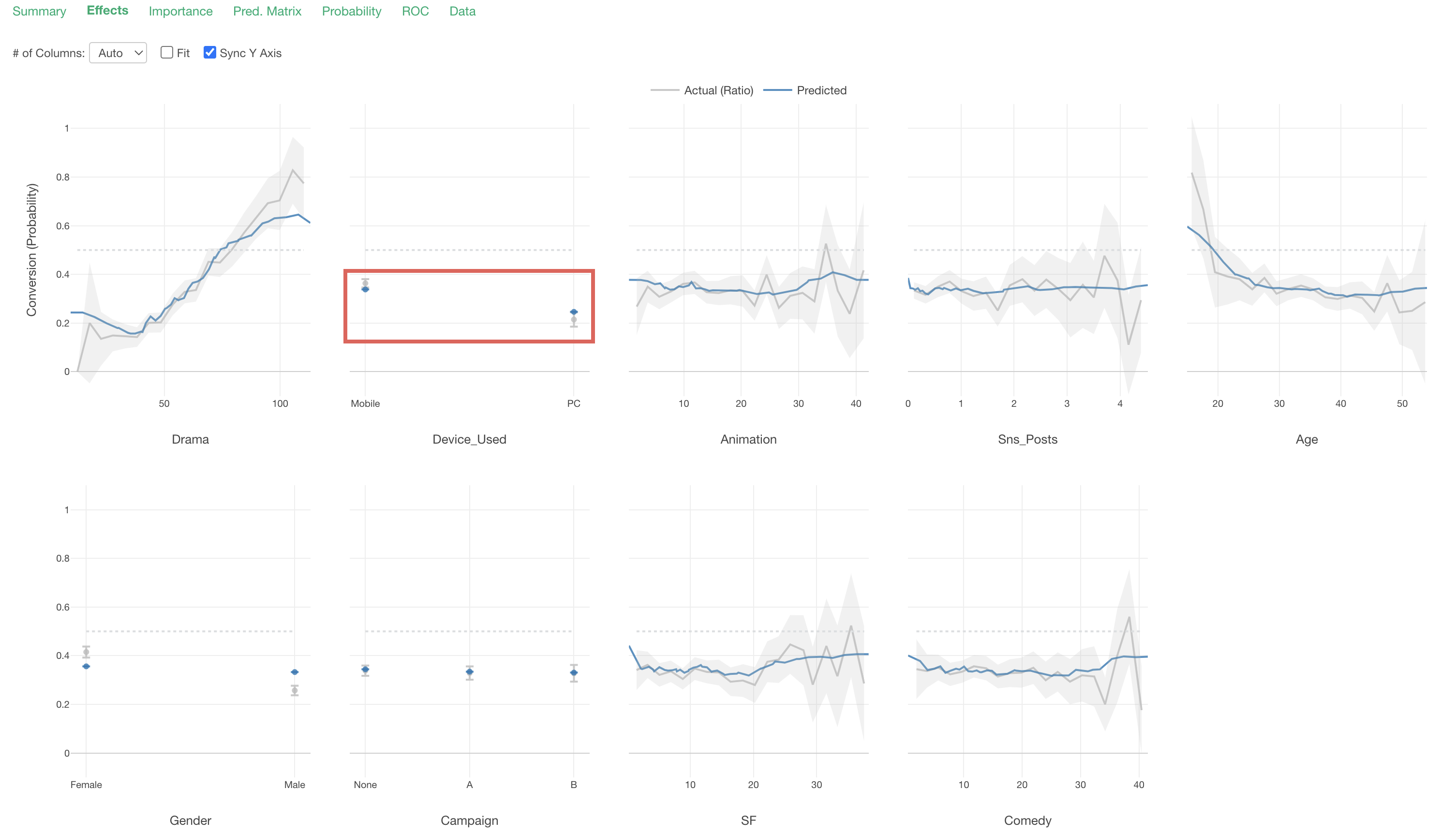
Looking at “Device_Used”, we can see that the conversion rate is higher for those whose main device is “Mobile” compared to “PC.”

Summary

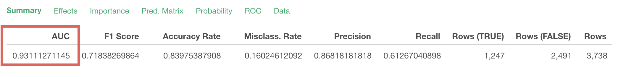
In the Summary tab, you can check the evaluation of this prediction model.

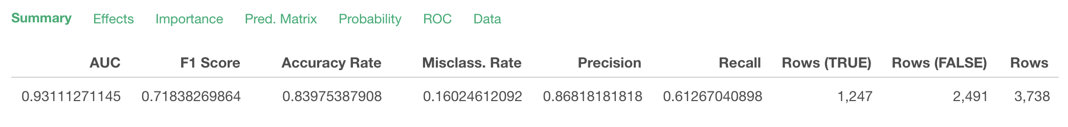
How well this model can separate TRUE and FALSE for conversion is expressed by the “AUC” metric, and you can check the detailed definition of the AUC metric from the information icon.

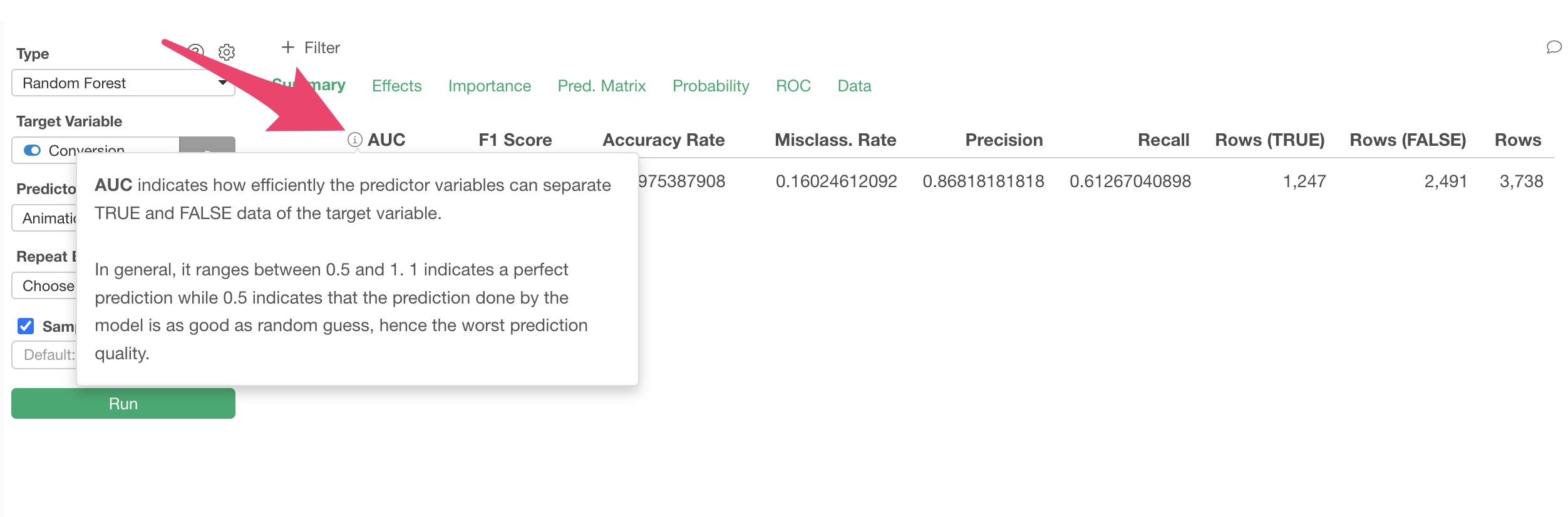
As shown in the popup, AUC takes values between 0.5 and 1. The closer to 1, the better the model is at separating “TRUE/FALSE.”

In this case, the AUC is 0.93, which is close to 1, so it seems that this model can separate TRUE and FALSE well.

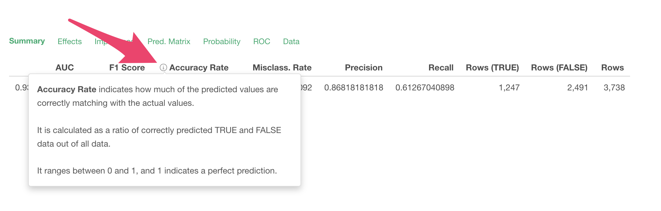
You can also check the definitions of several other metrics displayed in the Summary tab in the same way.

In this trial tour, we introduced how to interpret Random Forest, but in Exploratory, you can interpret any type of prediction model based on the “Grammar of Analytics” mechanism.

For details on the Grammar of Analytics, please refer to this note.

Predicting Conversion for Prospects in Trial

Next, we will use the conversion prediction model to predict the probability of conversion for customers whose conversion status is still unknown.

To predict new data using the created prediction model, you need data with the same columns as the predictor variables used in the created prediction model.

The new sample data for prediction can be downloaded from this page.

After downloading the trial status of new leads , open the downloaded folder and drag and drop it onto the Exploratory screen.

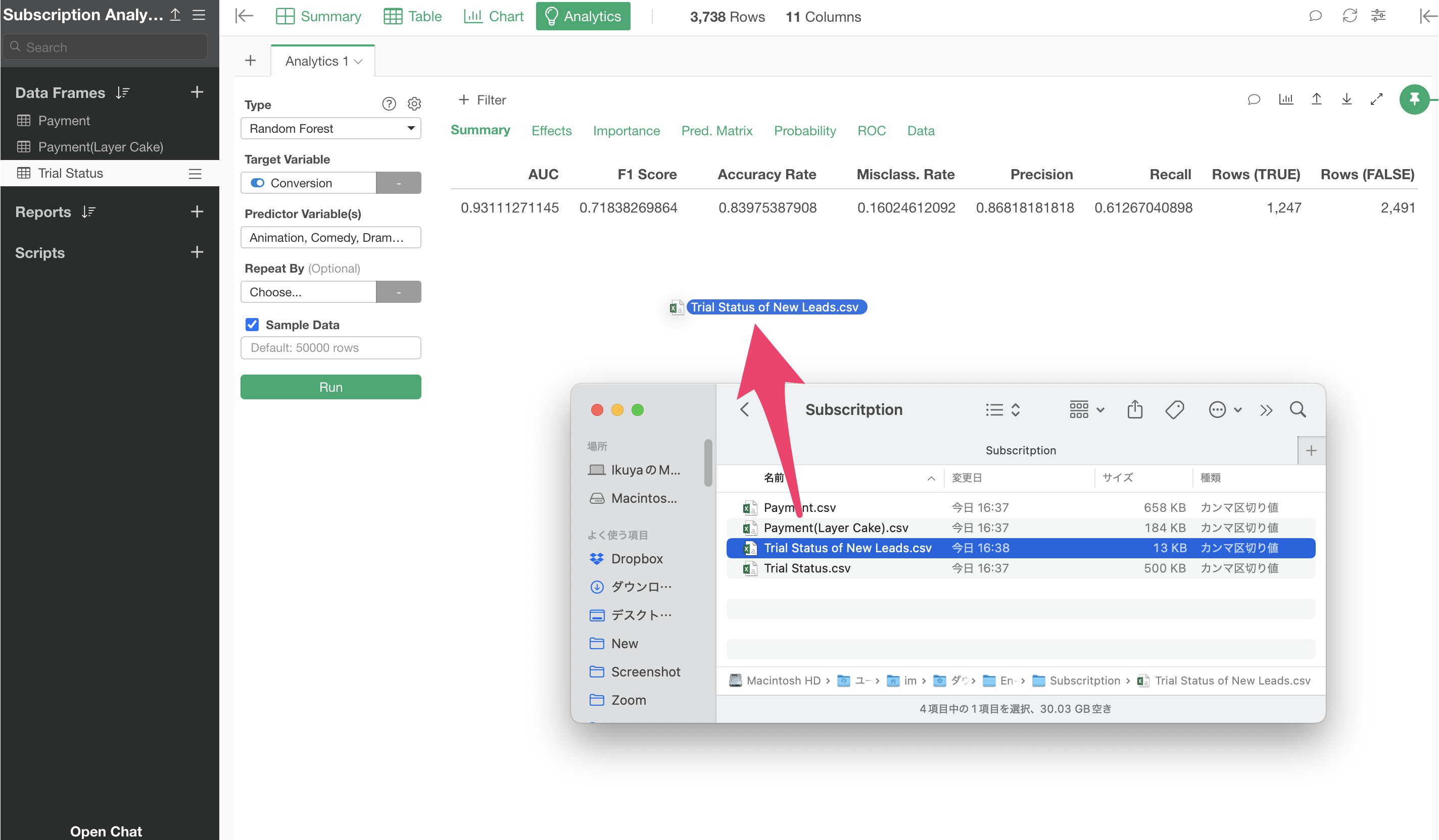
An import dialog will appear, so Import it.

A data frame settings dialog will appear, so click the “Create” button.

The trial status data for new prospects has been newly imported.

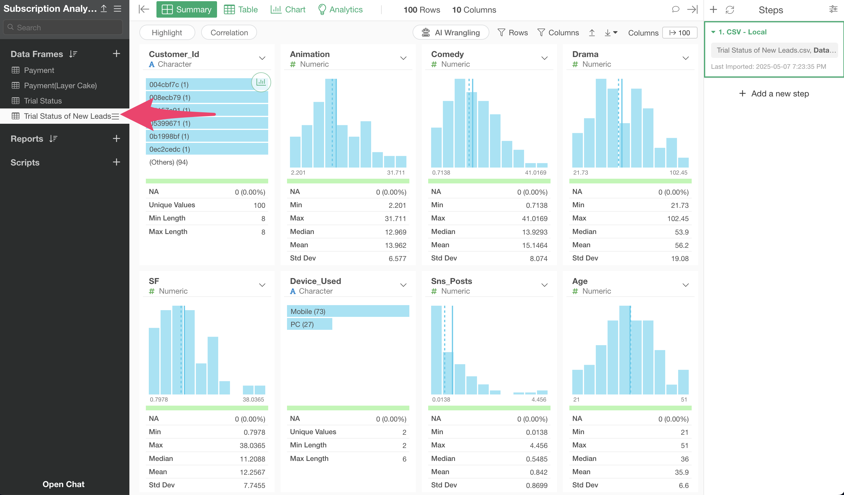
Now, we will use the created prediction model to predict conversion for the newly imported data.

Move to the Table View.

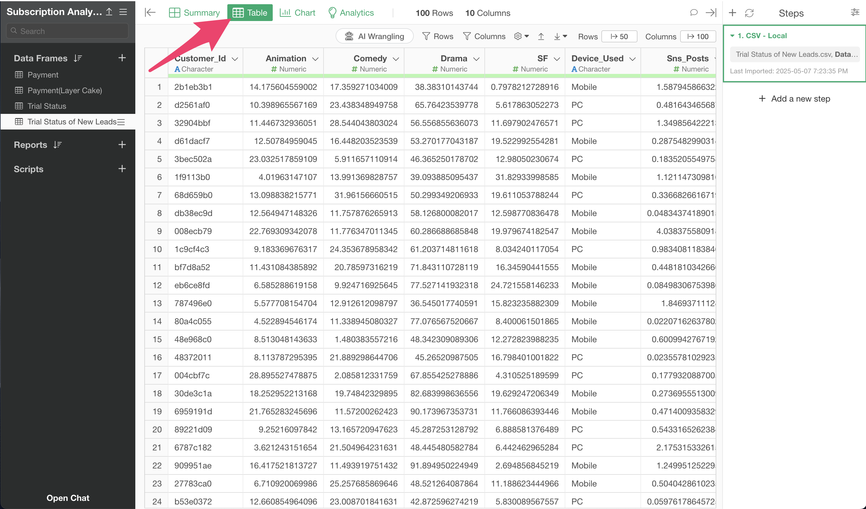
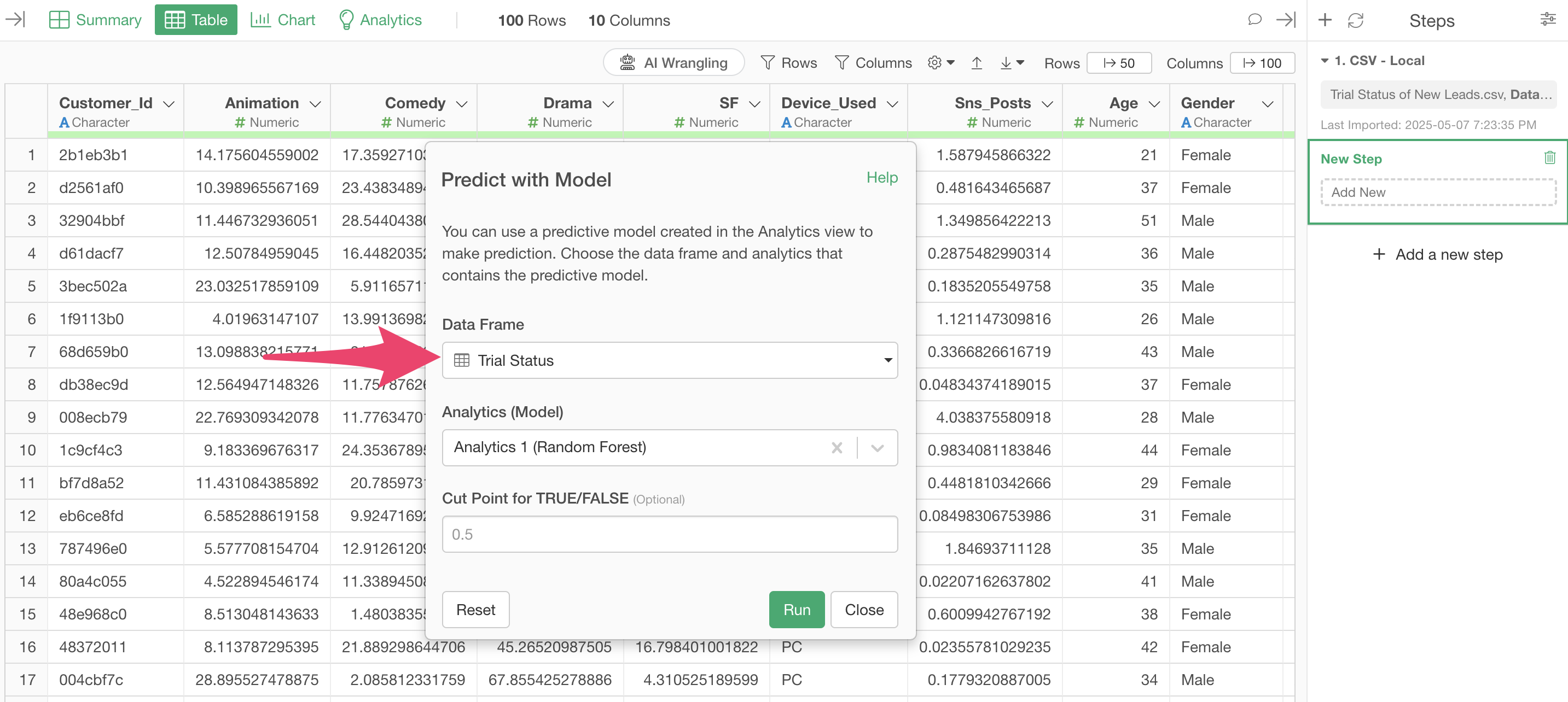
From the step menu, select “Predict with Model (Analytics View)”.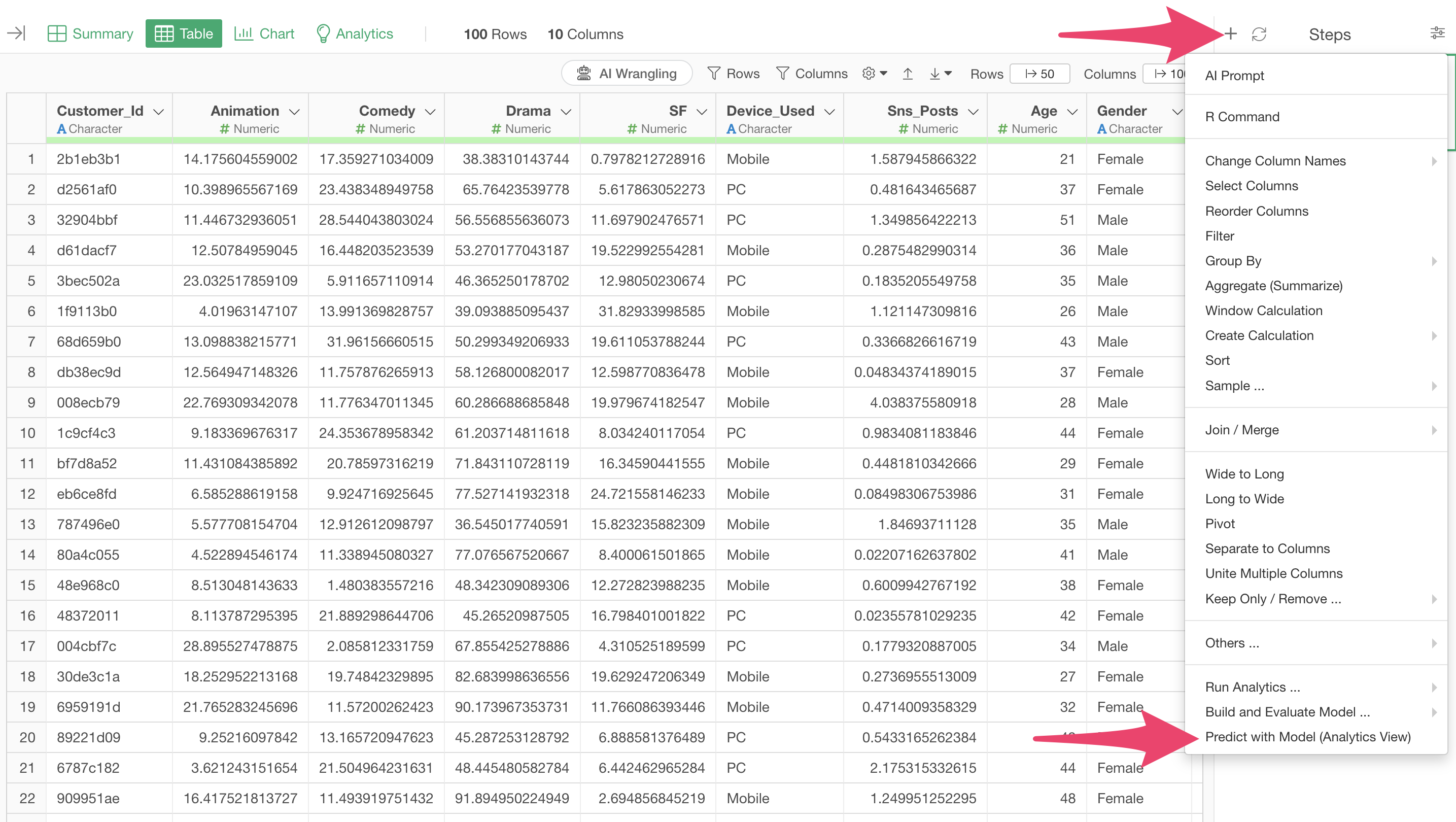

Selecting this menu allows you to use a prediction model created in another data frame to predict for the currently open data frame.

A “Predict with Model” dialog will appear, so select the data frame you want to use for prediction.

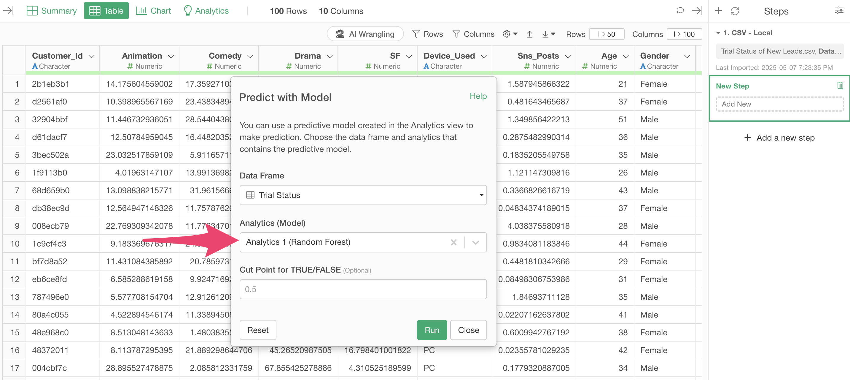
This time, we want to predict using the prediction model created in the “Trial Status” data frame, so select it for “Data Frame.”

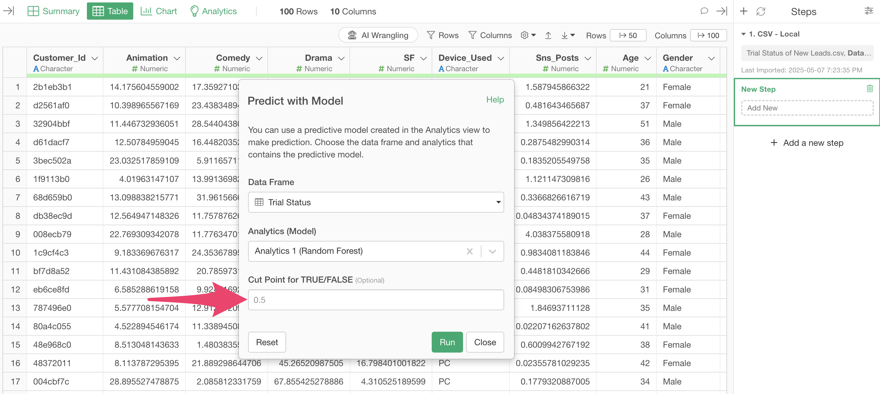
Next, select the model you want to use for prediction from “Analytics (Model)”.

This time, we will run with the default “TRUE/FALSE threshold” of 0.5. This will add a column that returns “TRUE” if the probability returned by the prediction model is 0.5 (50%) or higher, and “FALSE” if it is less than that.

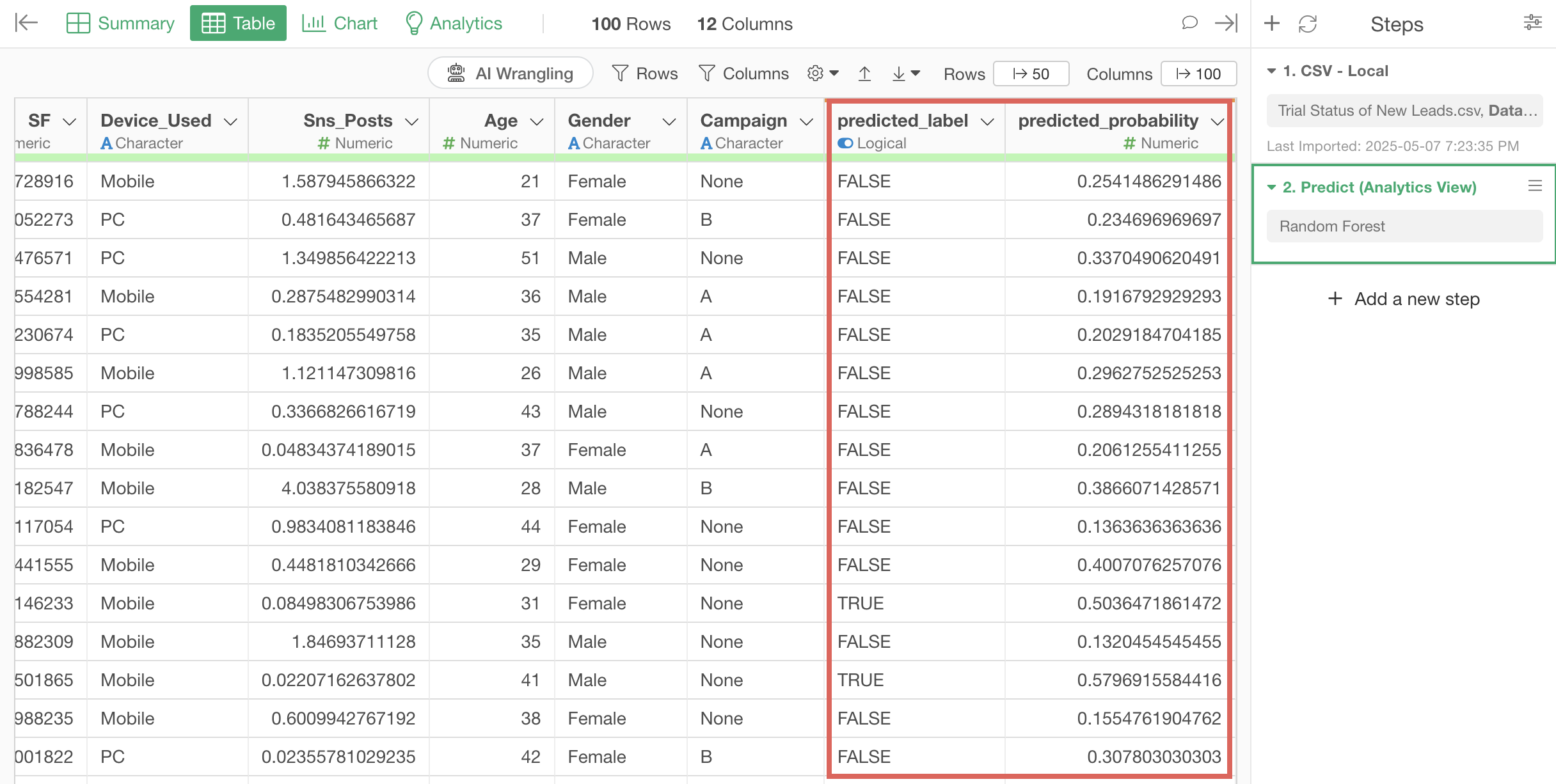
A step to predict conversion has been added, and columns for the probability of conversion “predicted_probability” and whether they will convert based on that probability and the set threshold “predicted_label” have been added to the data.

Subscription Data Analysis

Other parts of the trial tour for subscription-based business users can be found at the links below.

Visualizing Business KPIs - Link
Creating Layer Cake Charts - Link
Conversion Factor Analysis and Prediction
Cohort Analysis - Link

Next time, we will perform “Cohort Analysis” to examine whether retention is improving.

Like this time, it’s content that you can complete in about 20 minutes, so please give it a try!