Survey Data Analysis Part 3 - Factor Analysis
This note is the third installment, “Factor Analysis,” of the “Survey Data Analysis” trial tour designed to efficiently learn how to effectively utilize survey data to improve business and services.
Factor analysis is a statistical algorithm used to understand the background and motivations behind survey responses.
By conducting factor analysis, you can discover the commonalities behind survey responses, known as “factors,” which can be utilized for product development, targeting in marketing activities, and communication.
The estimated time required is about 20 minutes.
Let’s get started!!
What is Factor Analysis?
For example, a survey was conducted on “What People Want from Beer,”
and the following results were obtained.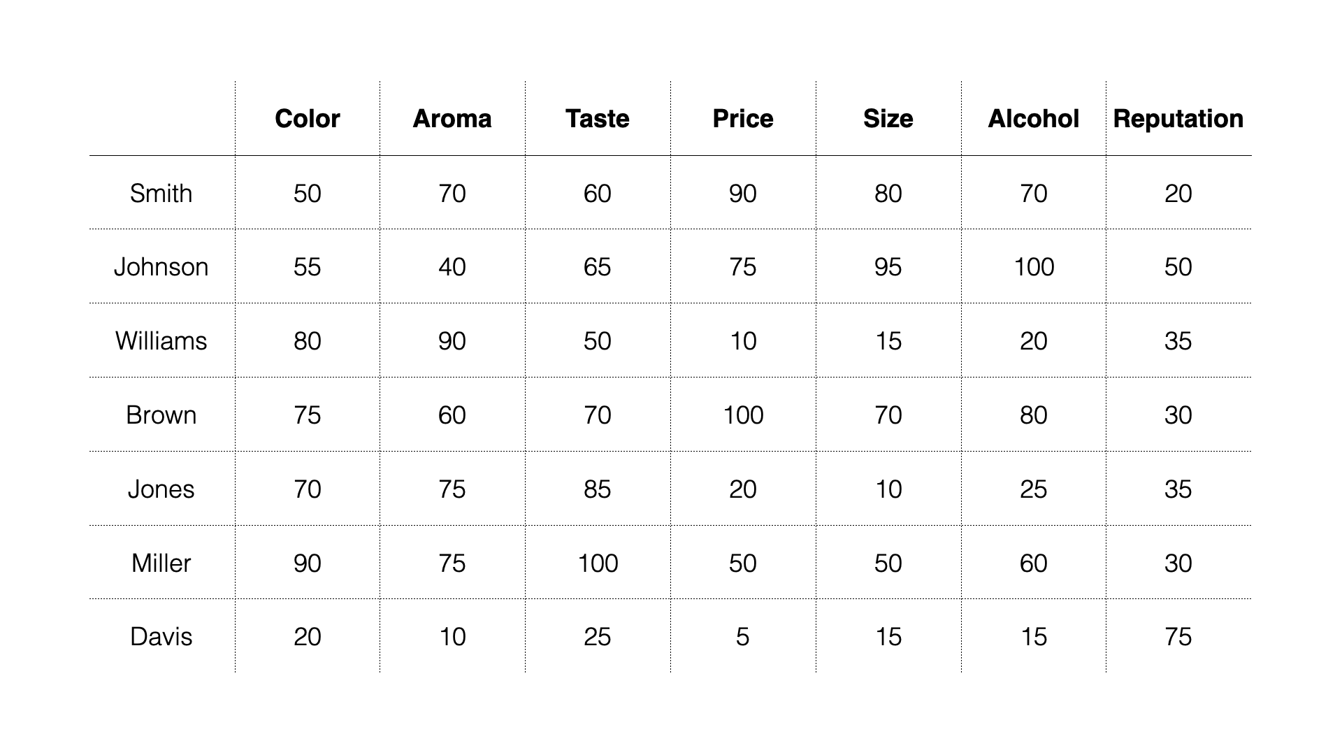 In
this data, each row represents one respondent, and each column
represents an importance score. The higher the value, the more important
that item is.
In
this data, each row represents one respondent, and each column
represents an importance score. The higher the value, the more important
that item is.
Looking at the responses, some people seem to prioritize “Price,”
“Size,” and “Alcohol.”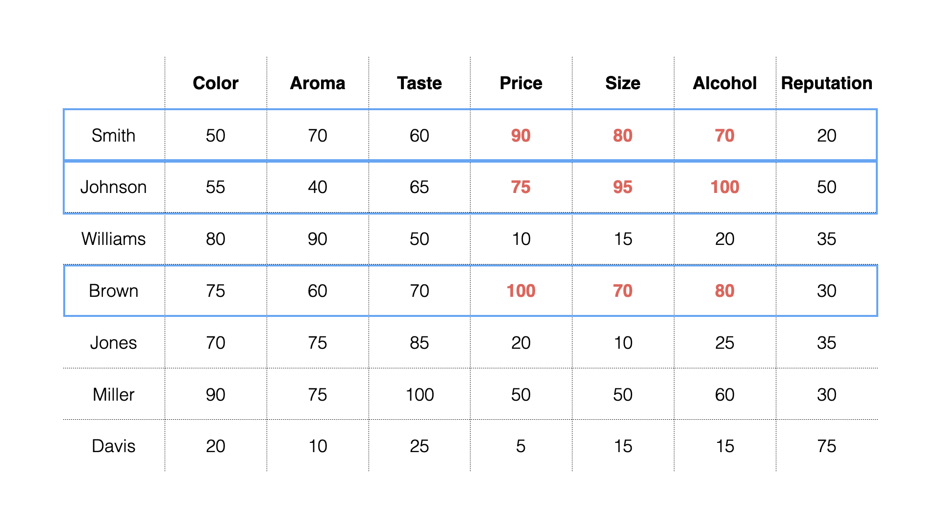 Others
prioritize “Color,” “Aroma,” and “Taste.”
Others
prioritize “Color,” “Aroma,” and “Taste.”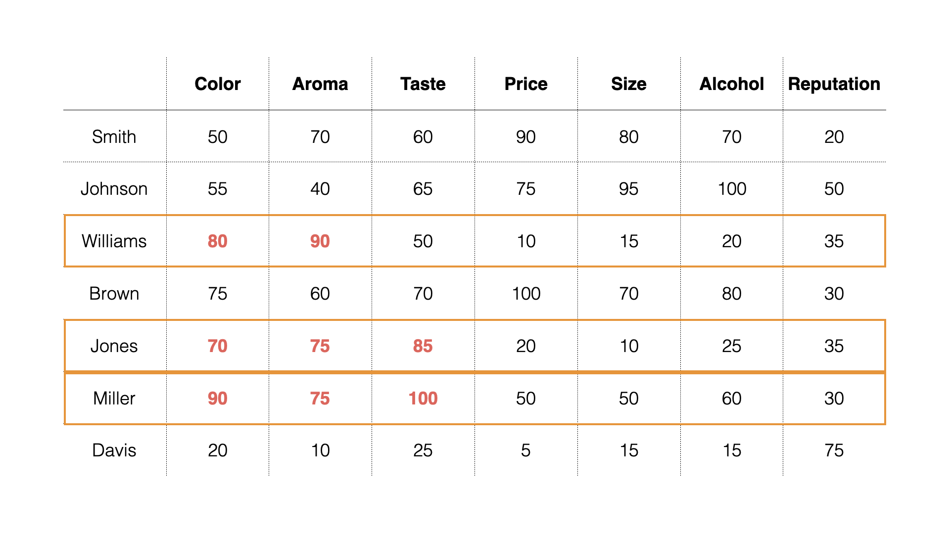 And
some prioritize “reputation.”
And
some prioritize “reputation.”

Each group considers different items important.
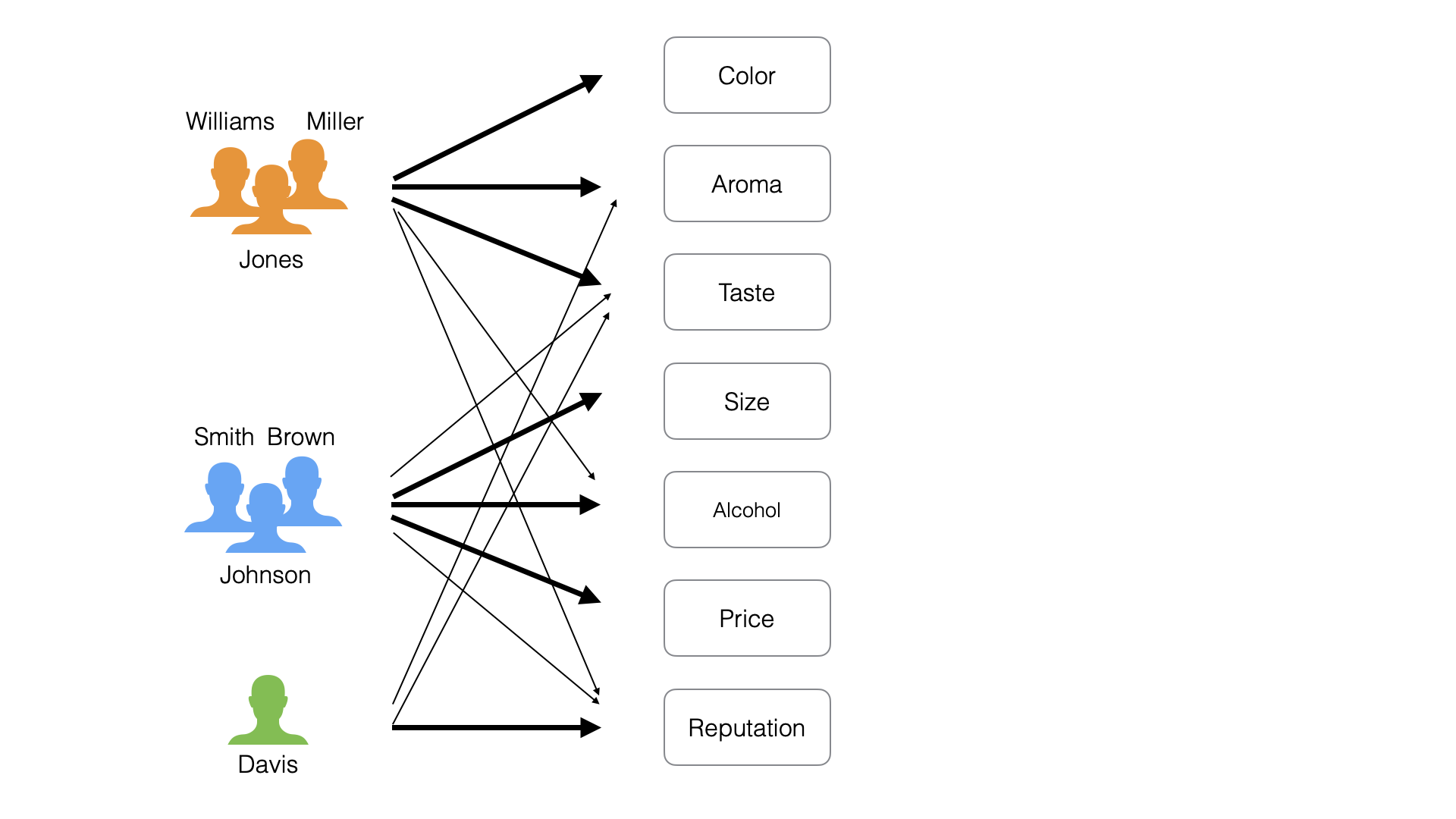
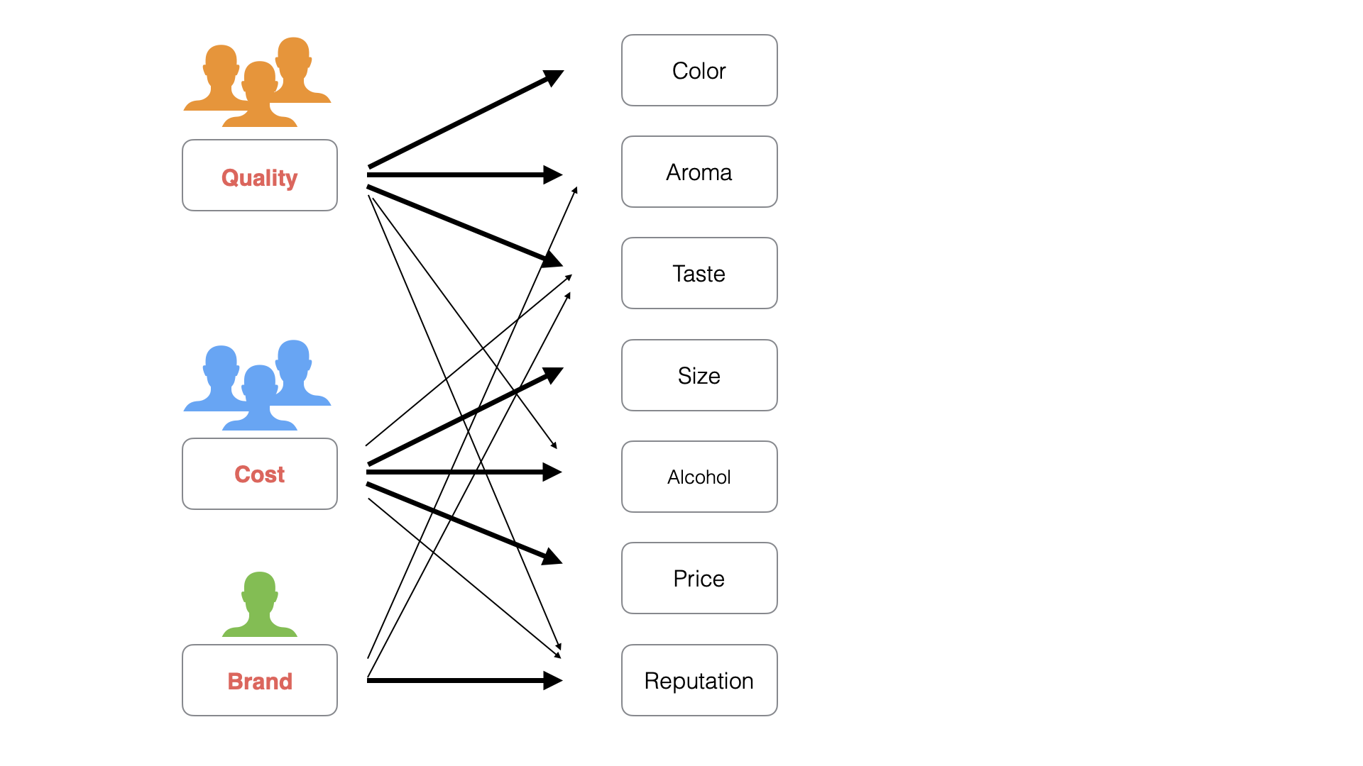
From another perspective, we can say there are different motivations (factors) that people consider important regarding “What People Want from Beer”:
- Orange people: “Quality”
- Blue people: “Cost”
- Green people: “Reputation”
 In
factor analysis, to enable such motivation labeling, motivations behind
survey responses are extracted as “factors,” and the strength of
correlation between each factor and each variable (question) is
calculated as a “factor loading.”
In
factor analysis, to enable such motivation labeling, motivations behind
survey responses are extracted as “factors,” and the strength of
correlation between each factor and each variable (question) is
calculated as a “factor loading.”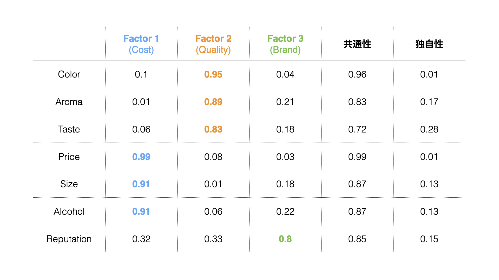 Factor
loadings take values between -1 and 1, with values closer to -1 or 1
indicating stronger influence of each factor on the respective
variables.
Factor
loadings take values between -1 and 1, with values closer to -1 or 1
indicating stronger influence of each factor on the respective
variables.
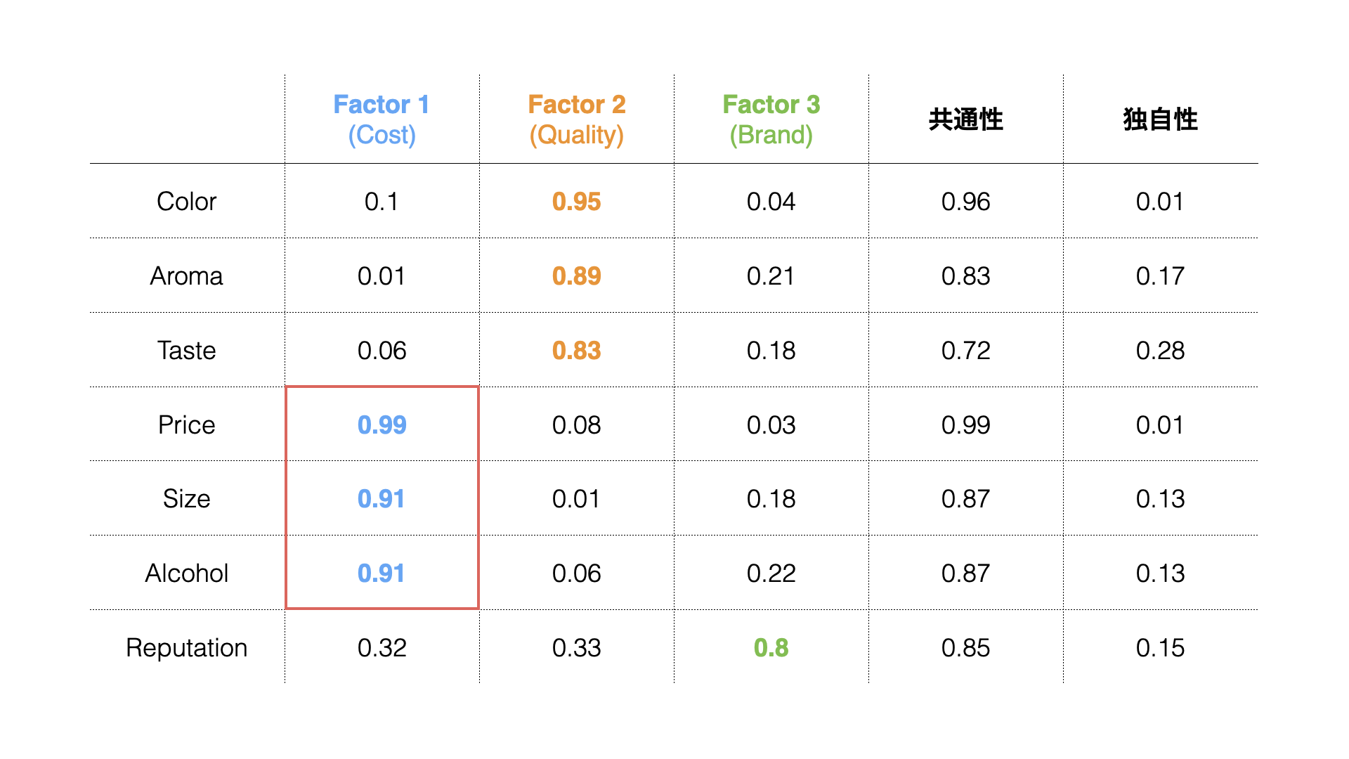
Therefore, for example, since “Factor 1” has high “factor loadings” for “Price,” “Size” and “Alcohol,” it has a strong relationship with Factor 1, and Factor 1 can be named “Cost.”
Required Data
Factor analysis requires data where each row represents one observation (e.g., respondent), and numerical columns are necessary for factor extraction.

Data Overview
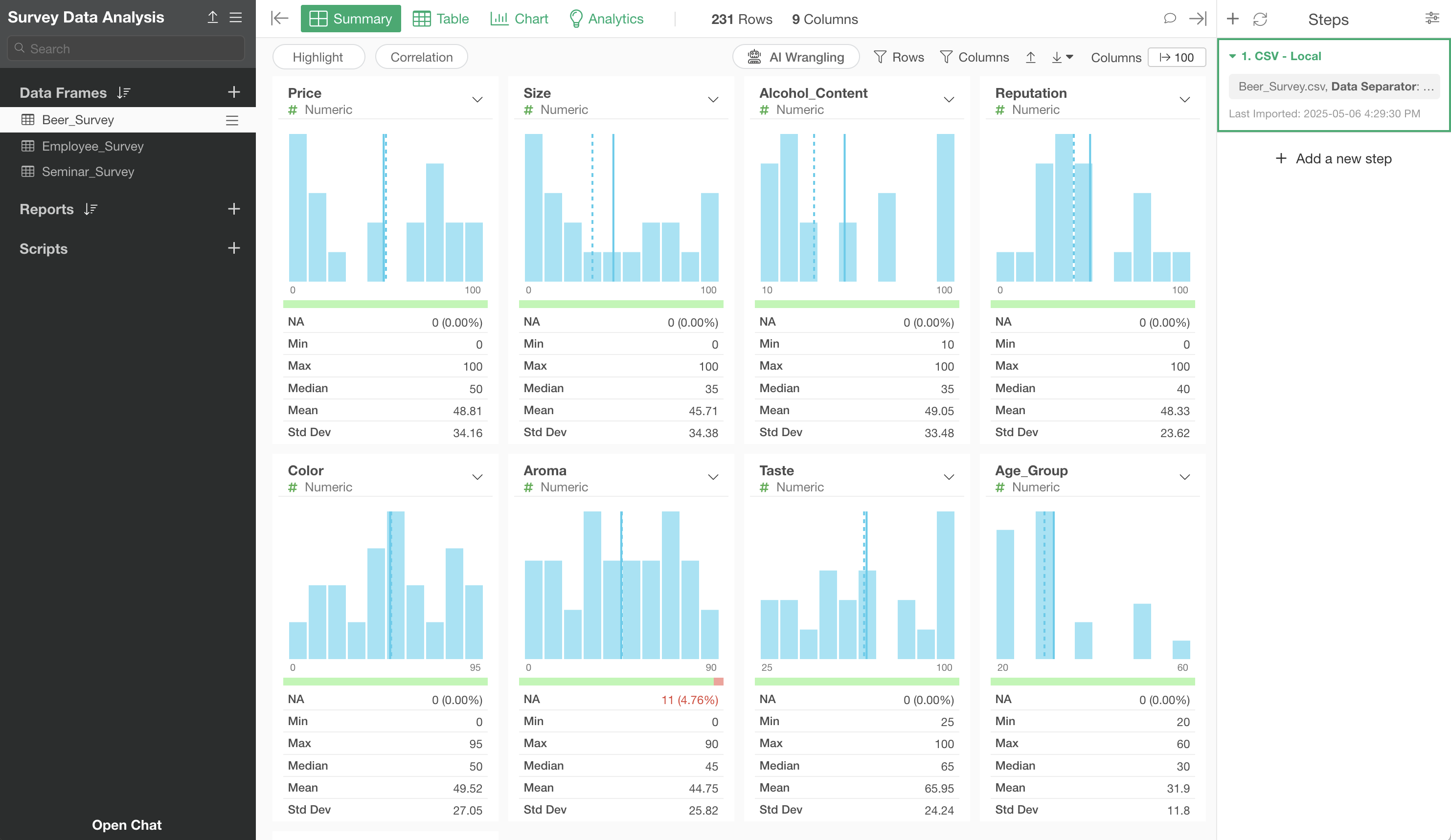
For this exercise, we’ll use sample data from a survey about “What People Want from Beer.”
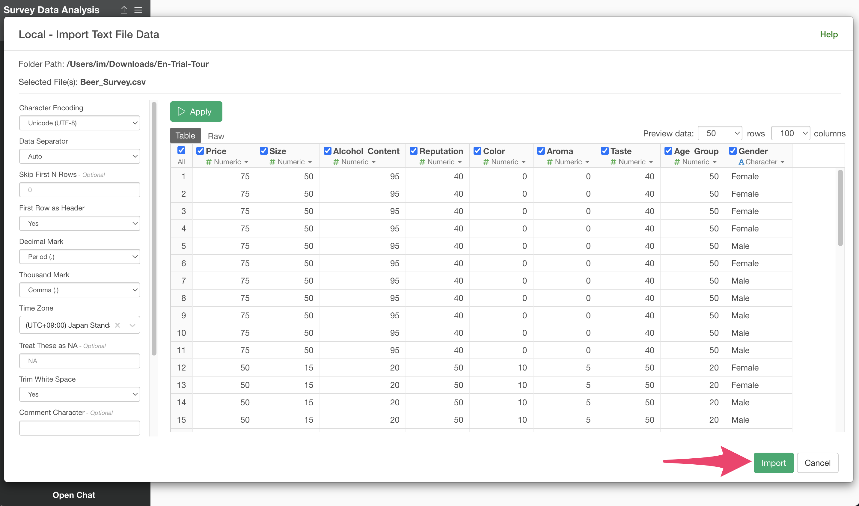
In this data, each row represents one respondent, and the columns contain response scores for questions about price and size, as well as respondent attributes (Age group, Gender).
The response scores are on a 100-point scale, with higher values indicating higher importance.
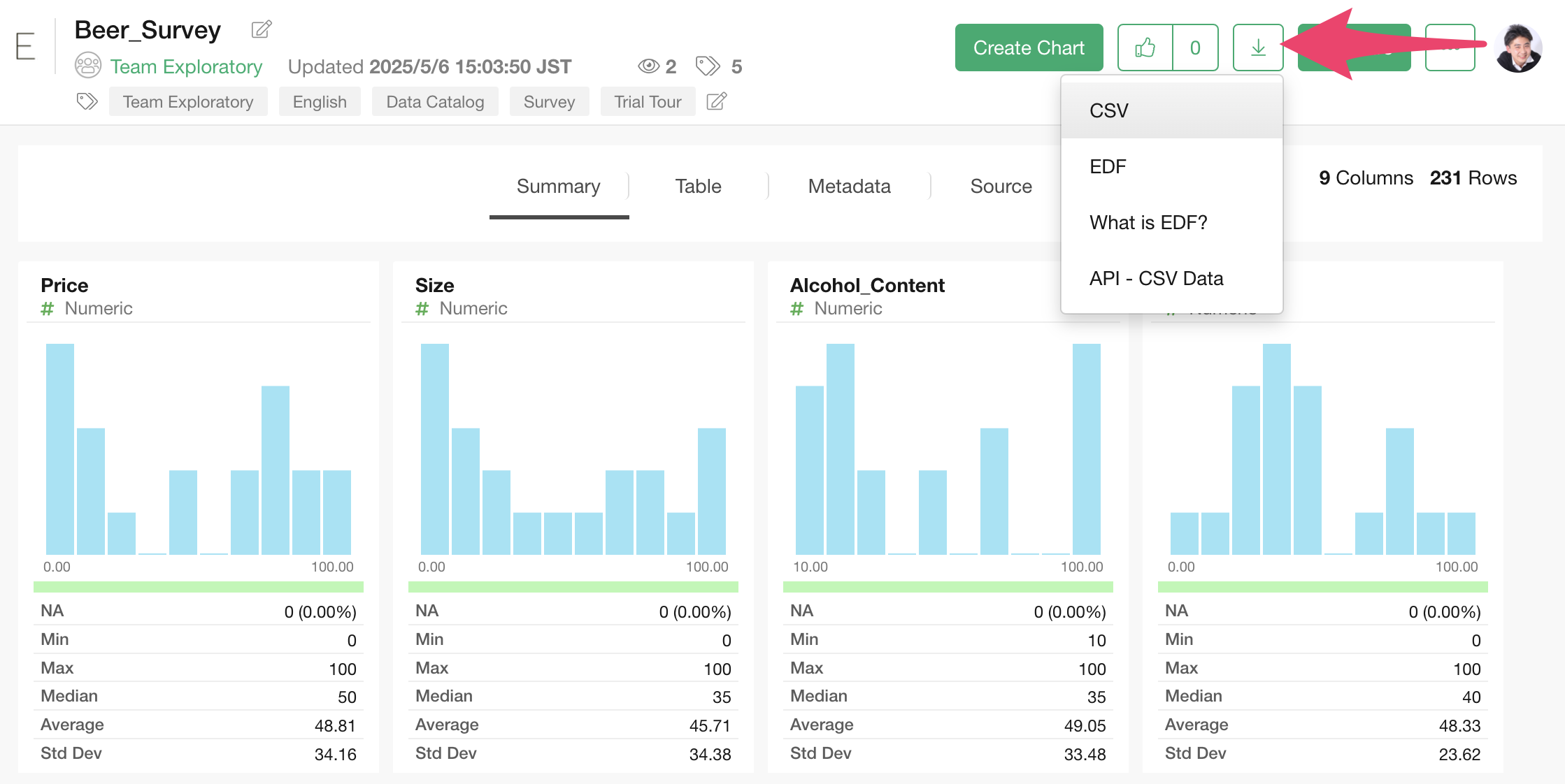
Importing Data
The data can be downloaded from this page.
 Once
you’ve downloaded the customer trial status data, open the downloaded
folder and drag and drop onto the Exploratory screen.
Once
you’ve downloaded the customer trial status data, open the downloaded
folder and drag and drop onto the Exploratory screen.
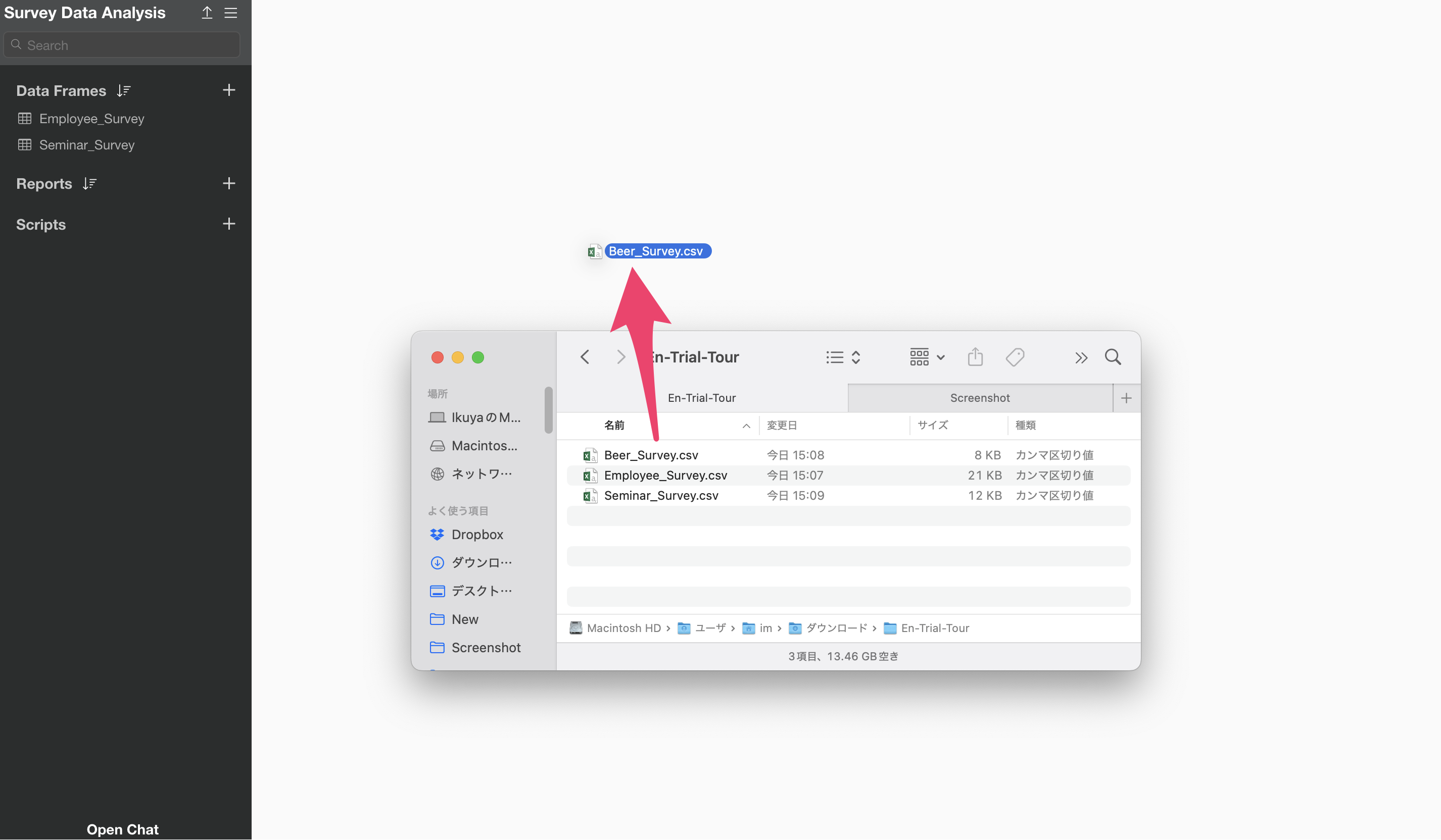
An import dialog will appear.
In the import dialog, you can specify settings for importing data from the items on the left, but since no settings are needed this time, click the “Import” button.
A data frame settings dialog will appear, so click the “Create” button.
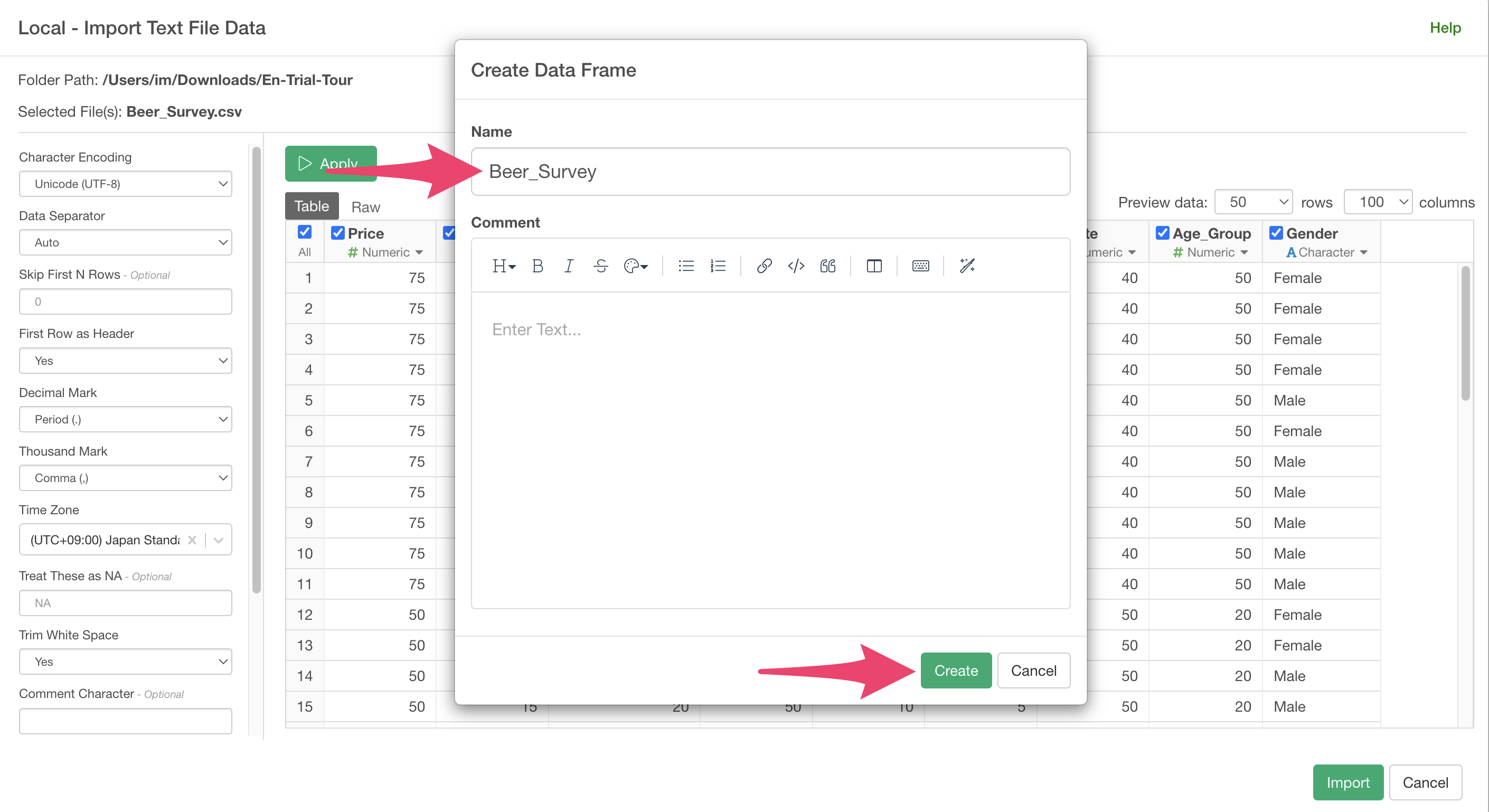
The beer survey data has been imported.
Running Factor Analysis
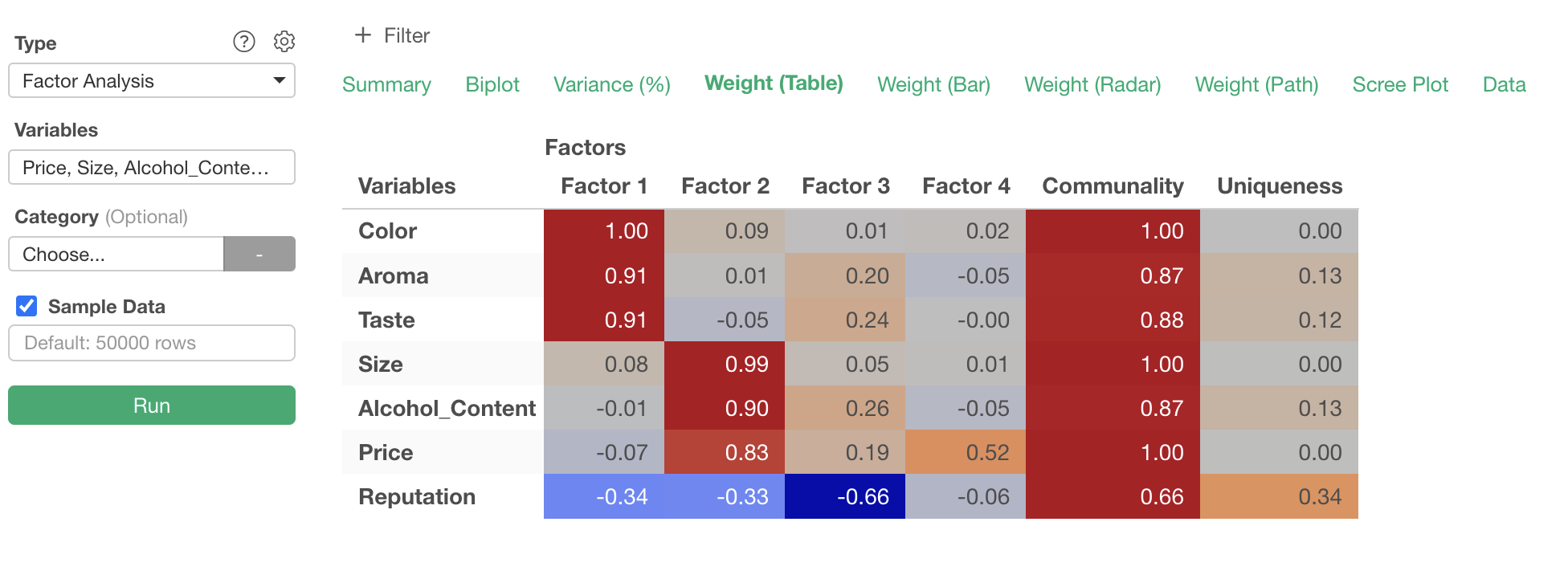
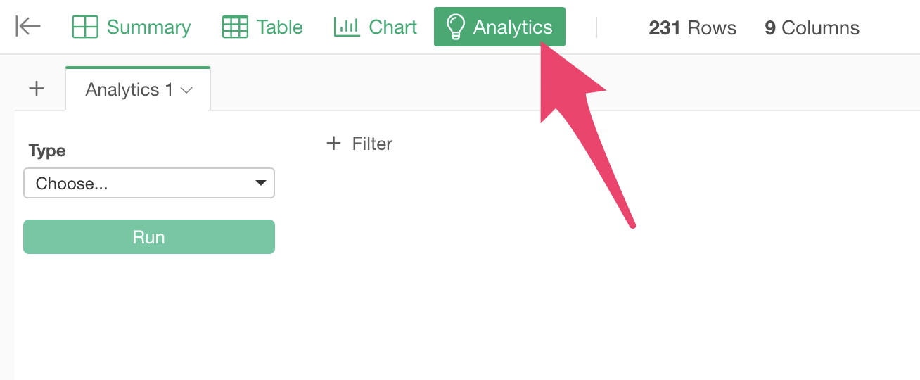
To perform factor analysis, move to the “Analytics View.”
Select “Factor Analysis” as the type.
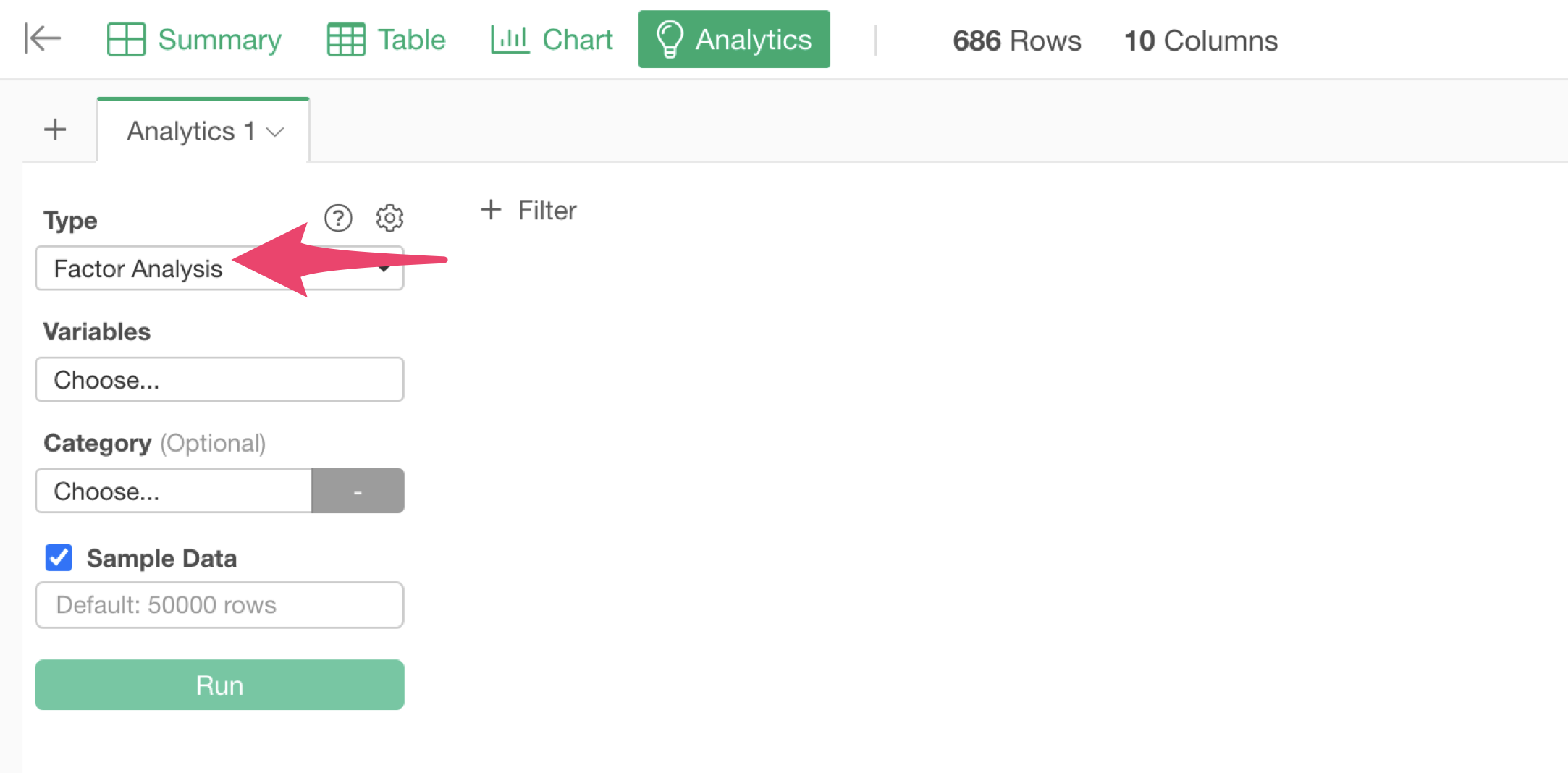
Click on the variable columns to select the columns to use for factor analysis. You can select multiple columns at once by holding down the Shift key.
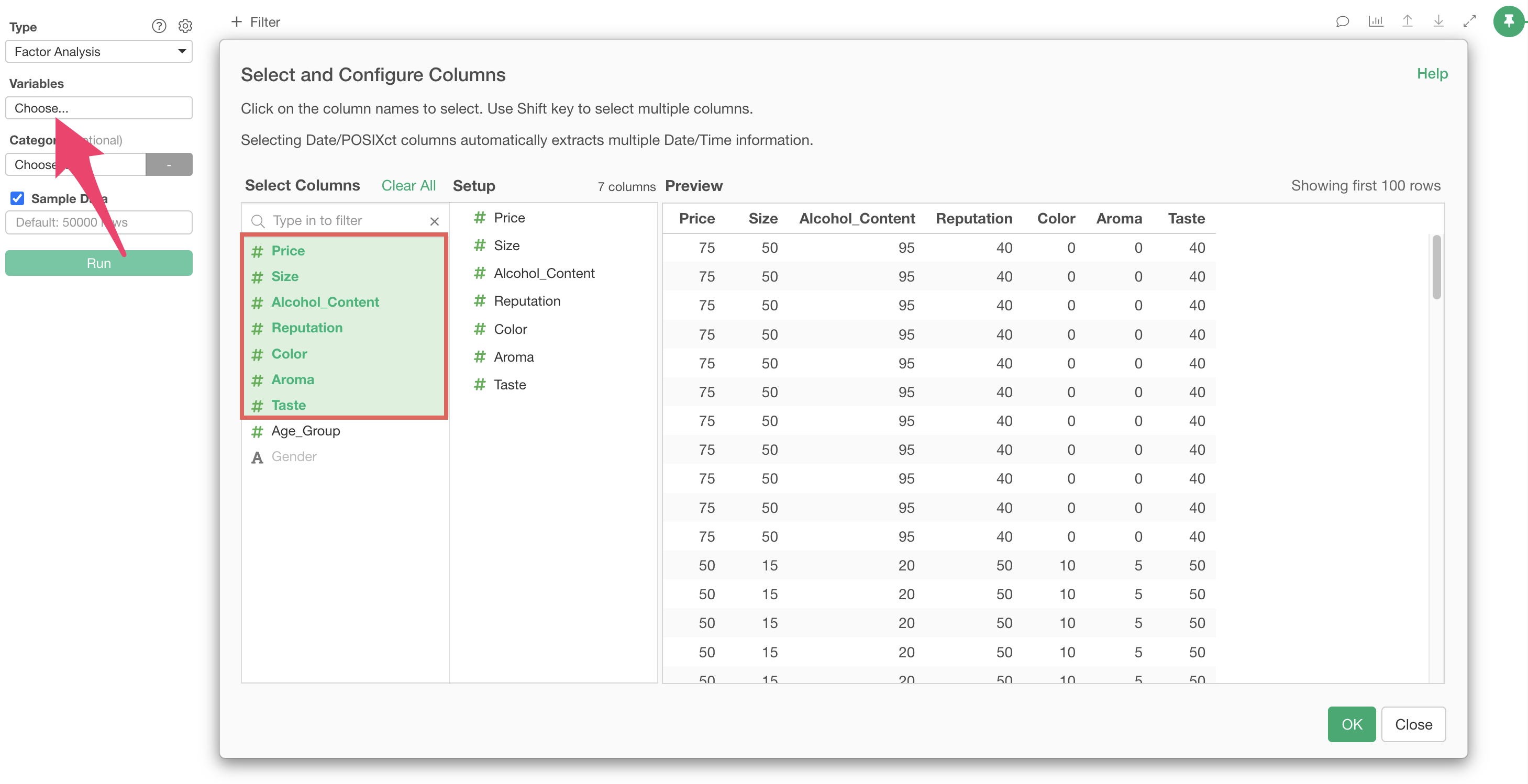
After specifying the columns, run the analysis to display the factor analysis results.
Interpreting the Results
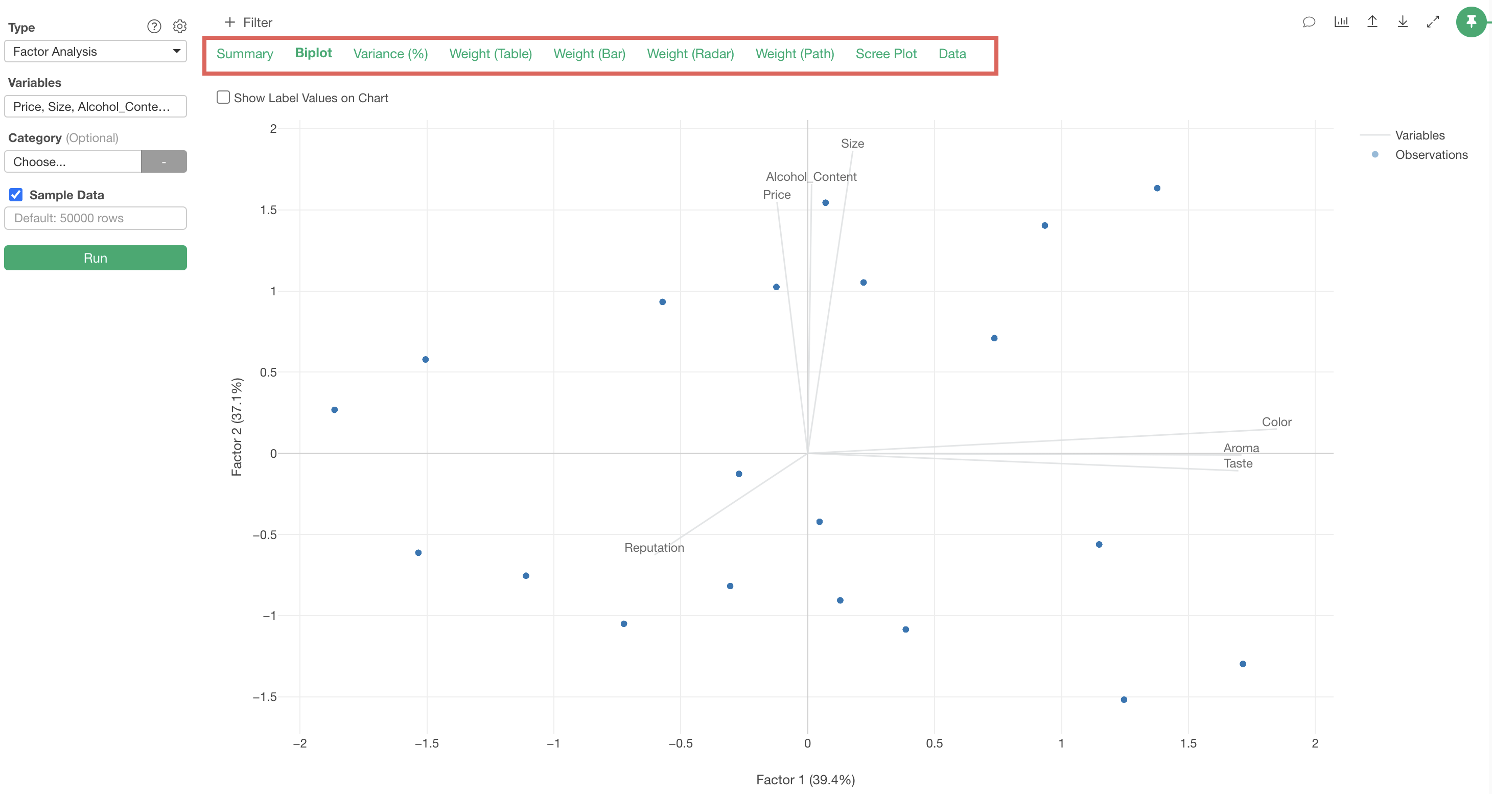
When you run factor analysis, multiple tabs are displayed to help interpret the results.
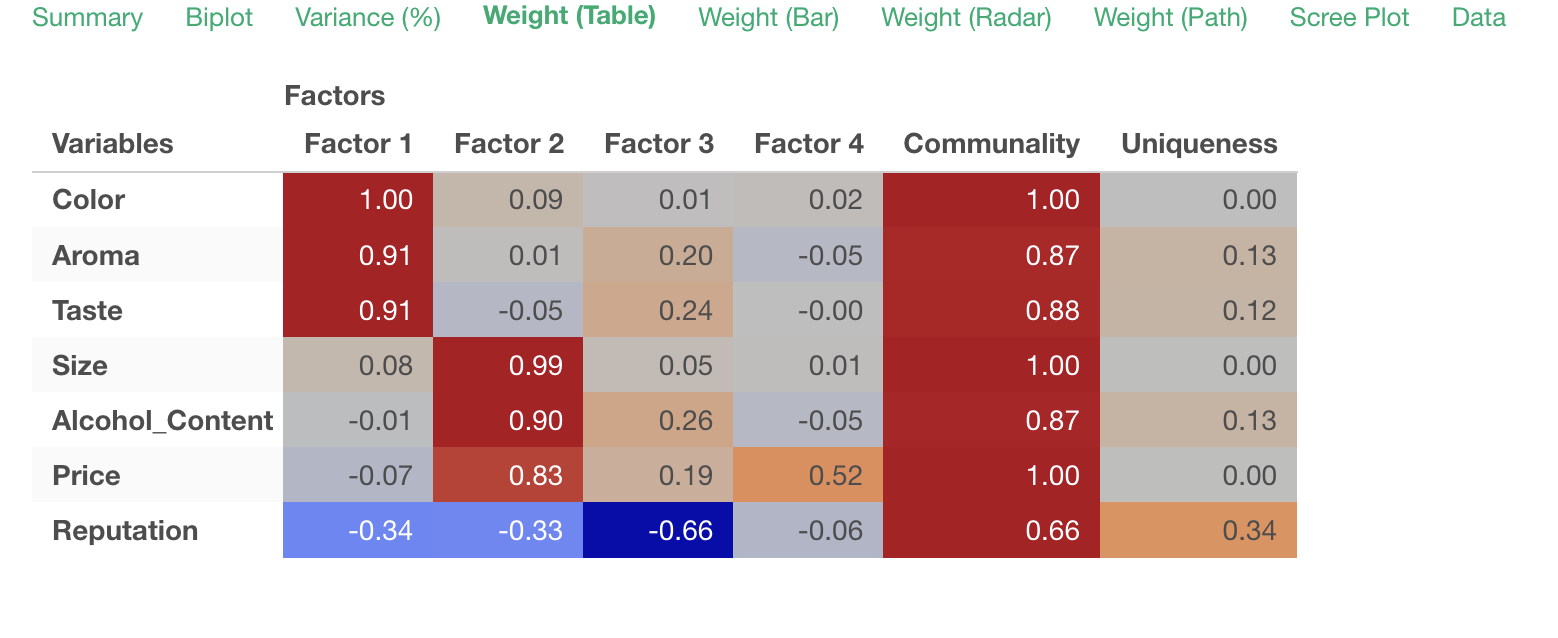
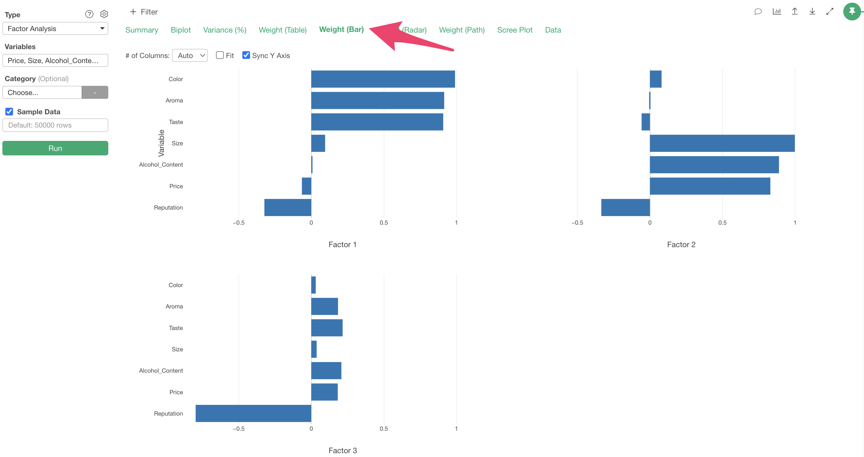
Weight (Table)
In the Weights (Table) tab, “factor loadings” are displayed for each extracted factor, showing the strength of influence each factor has on each variable (question).
Factor loadings take values between -1 and 1, with values closer to -1 or 1 indicating stronger influence of each factor on the respective variables.
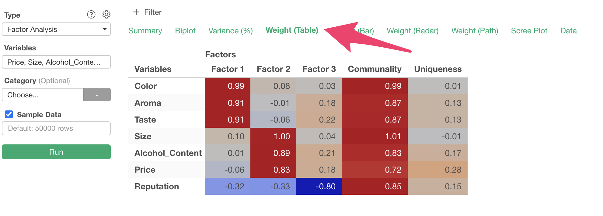
For example, considering variables with high factor loadings, we can identify commonalities like “Quality” for the first factor, where “Color,” “Aroma,” and “Taste” have factor loadings close to 1.
Similarly, we can name each factor as follows:
- Factor 1: Quality
- Factor 2: Cost
- Factor 3: Reputation
The same information can be confirmed in the Weight (Bar) tab,
and in the Weights (Radar) tab.
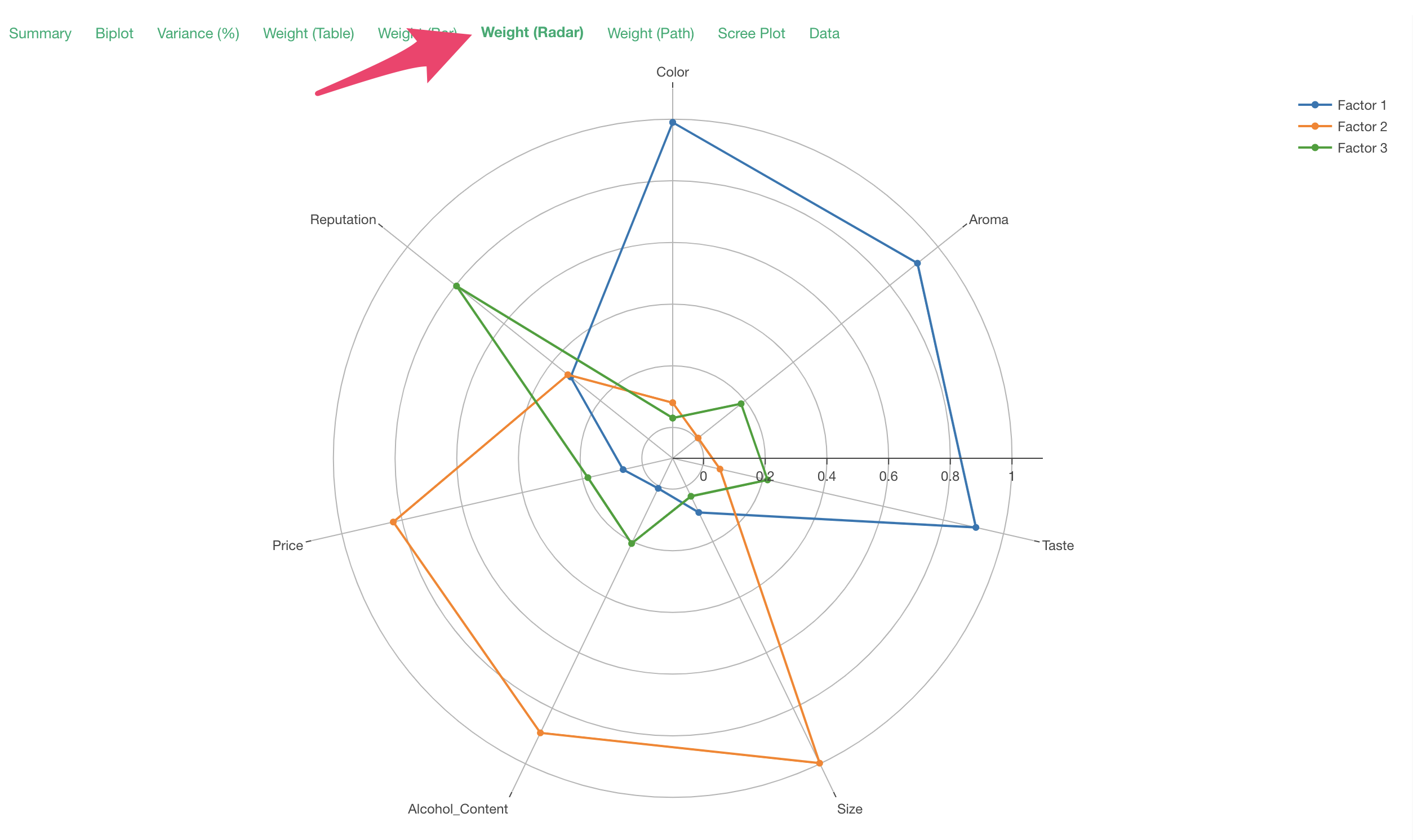
Note that the factor loadings displayed in the radar chart are the absolute values of the factor loadings.
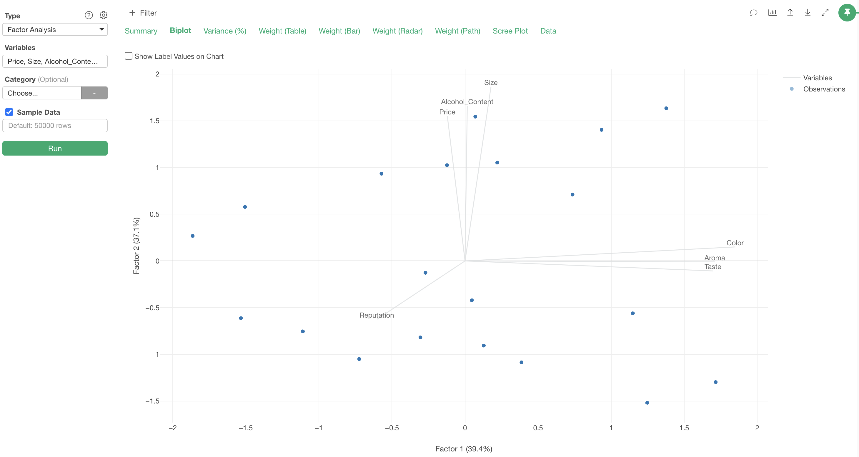
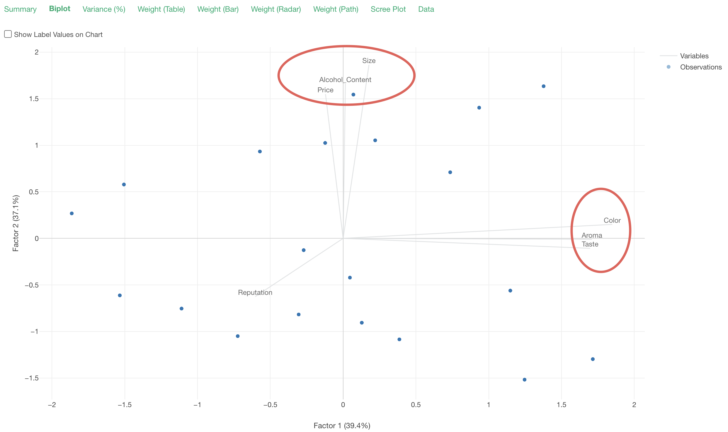
Biplot
In the “Biplot” tab, a chart is displayed that visualizes the relationships between the original variables based on the first two factors (Factor 1 on the X-axis and Factor 2 on the Y-axis).
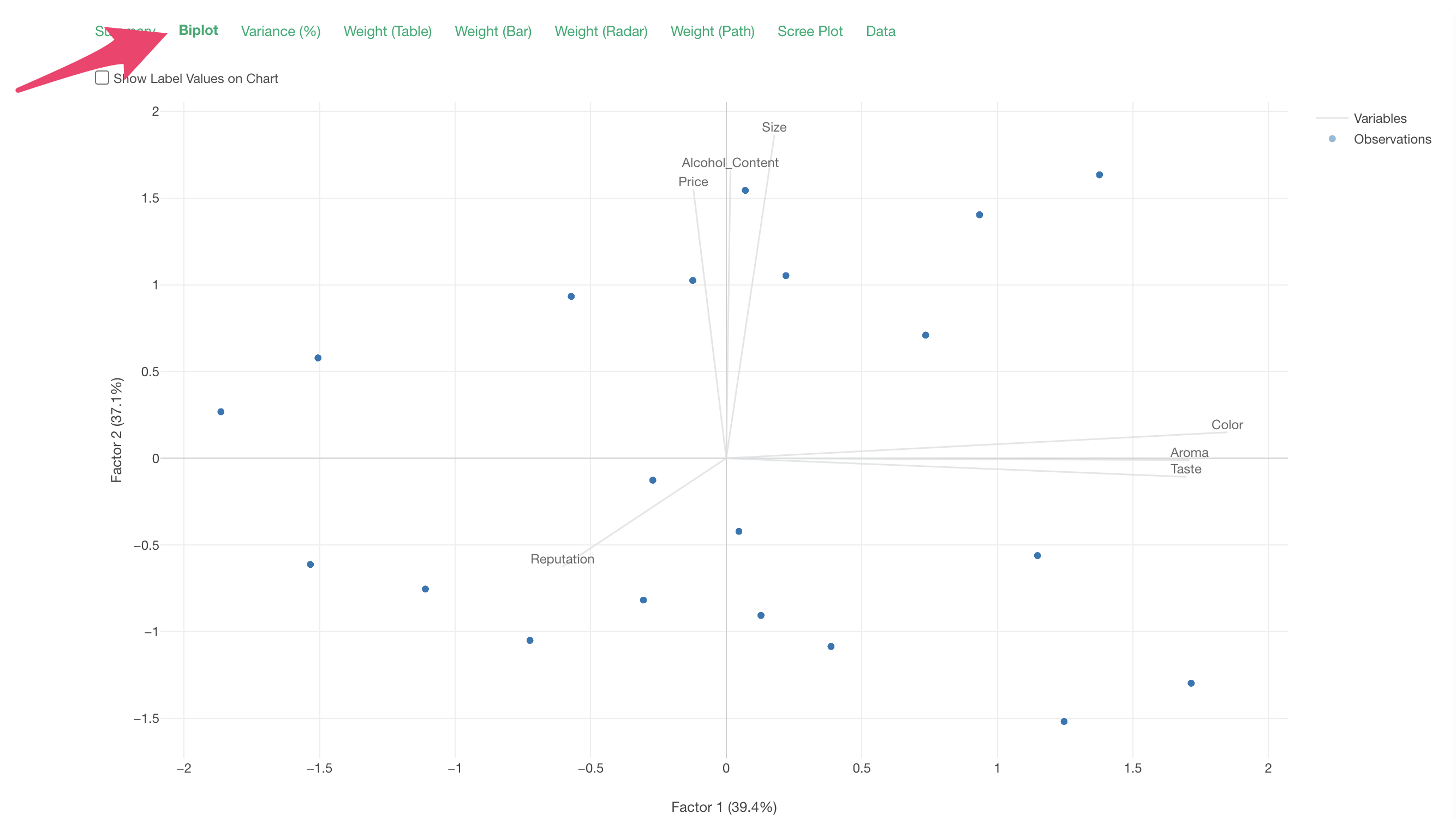
In the biplot, each line represents a variable (question), and each point represents a row of data (respondent). Also, lines of variables with strong correlations extend in the same direction.
Therefore, we can confirm the correlations between responses related to “Size,” “Alcohol_Content,” and “Price,” and the correlations between responses related to “Color,” “Aroma,” and “Taste.”
Scree Plot
The scree plot visualizes the error variance (eigenvalues) as the number of factors increases. The optimal number of factors is where the decrease in error variance converges. Often, the optimal number of factors is when the eigenvalue falls below the reference value of “1.”
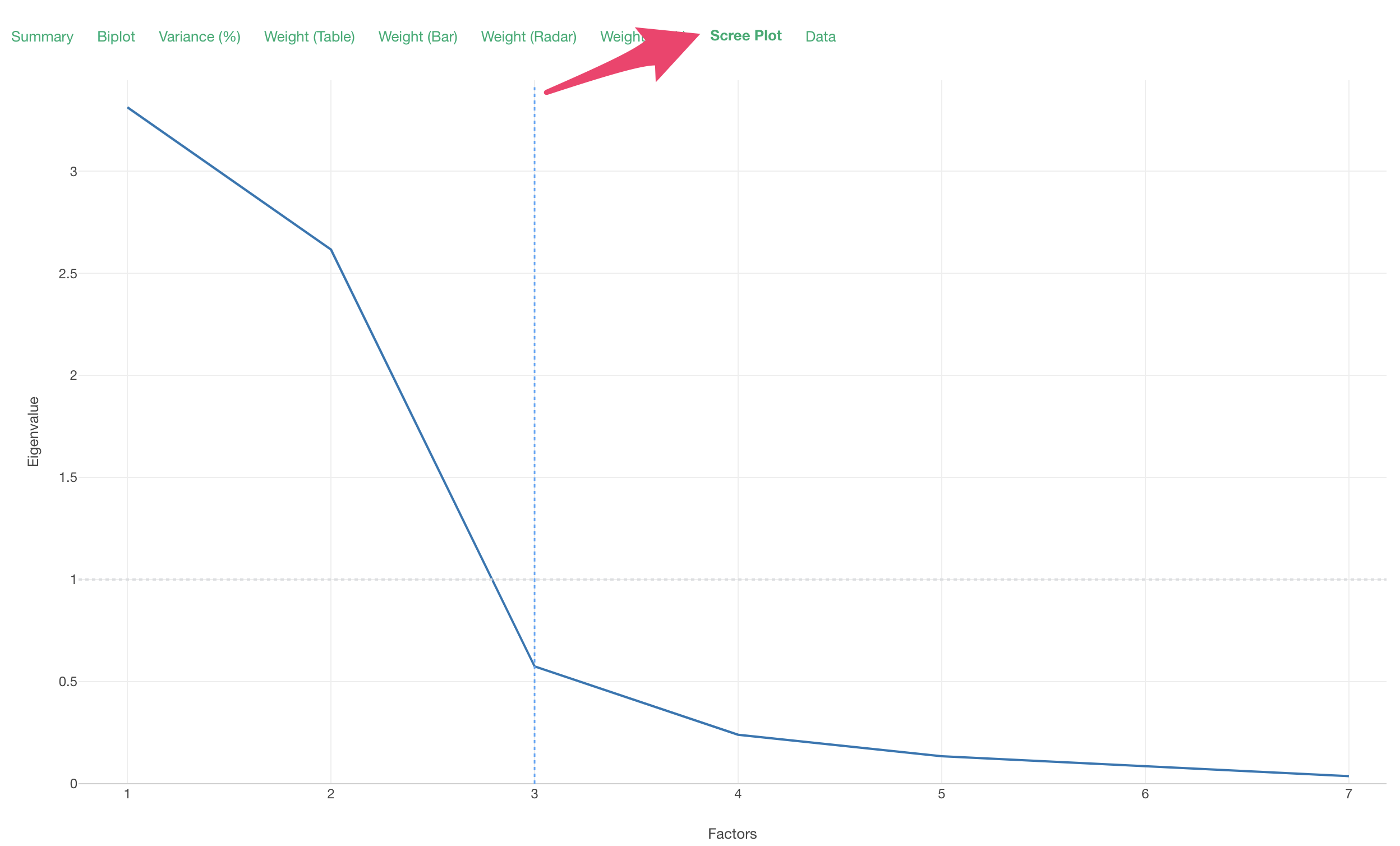
In this case, the Eigenvalues converge around 3, so the optimal number of factors is considered to be 3.
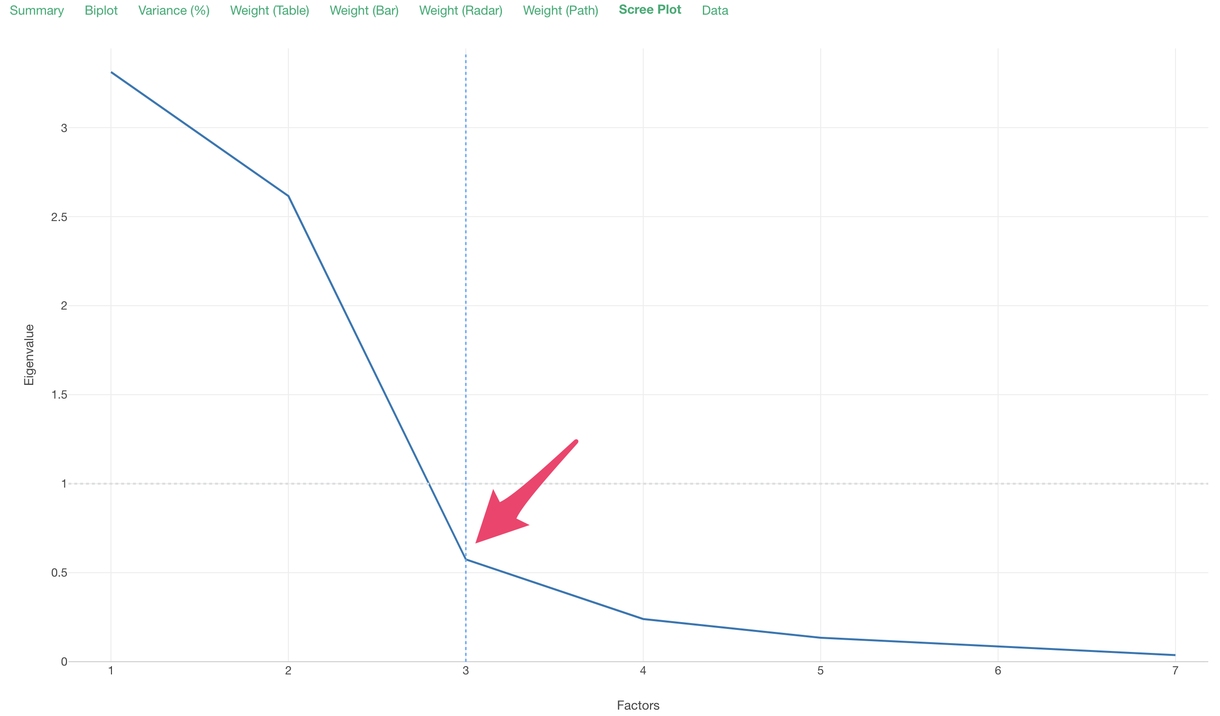
You can change the “Number of Factors” in the settings using the optimal number of factors explored in the scree plot.
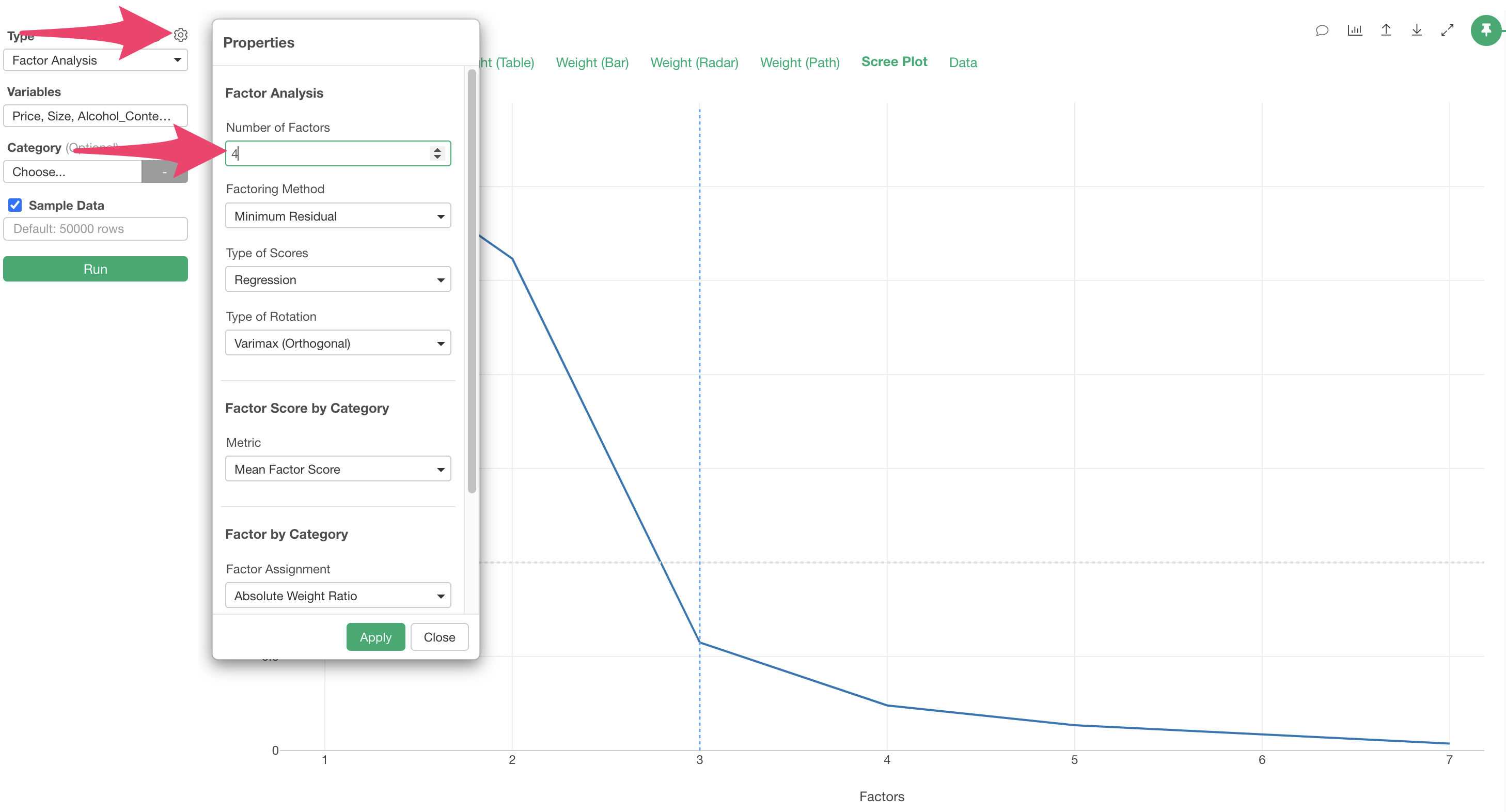
When you specify the number of factors, the execution results with the specified number of factors are displayed.