Does your data include Date and Time?
That’s great! You can analyze your data from many different perspectives.
But, of course, if you know how to work with Date and Time data.
In this post, I’m going to walk you through how you can address the following 5 common Date and Time data wrangling challenges in Exploratory.
- Convert Characters to Date & Time
- Extract Date & Time Attributes like January, Monday, etc.
- Calculate Duration Between Two Different Dates
- Filter Data based on Date & Time Values
- Round Date & Time Values
We are going to use the 2016 US Election TV Advertisement Campaign data, which was originally hosted at Political Ad Archive and I have cleaned up and shared it here. You can download it as either CSV or EDF (Exploratory Data Format) and import it into Exploratory.
Date and Time Data Type in R
Before we start, there is one thing to note. In R, there are two basic data types around date and time in R.
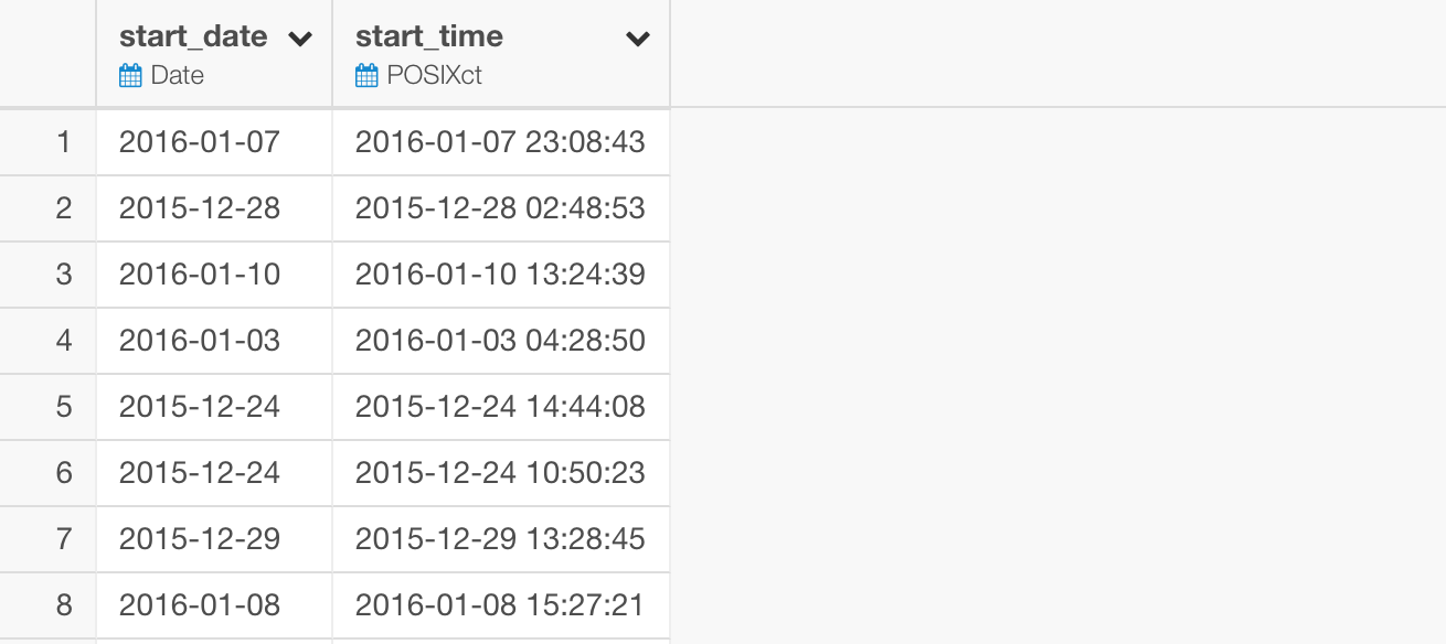
One is Date, which contains only the date information like 2016–01–10.
Another is POSIXct, which contains both date and time information like 2016–01–10 10:45:20.
Having said that, let’s begin.
1. Convert Characters to Date / Time
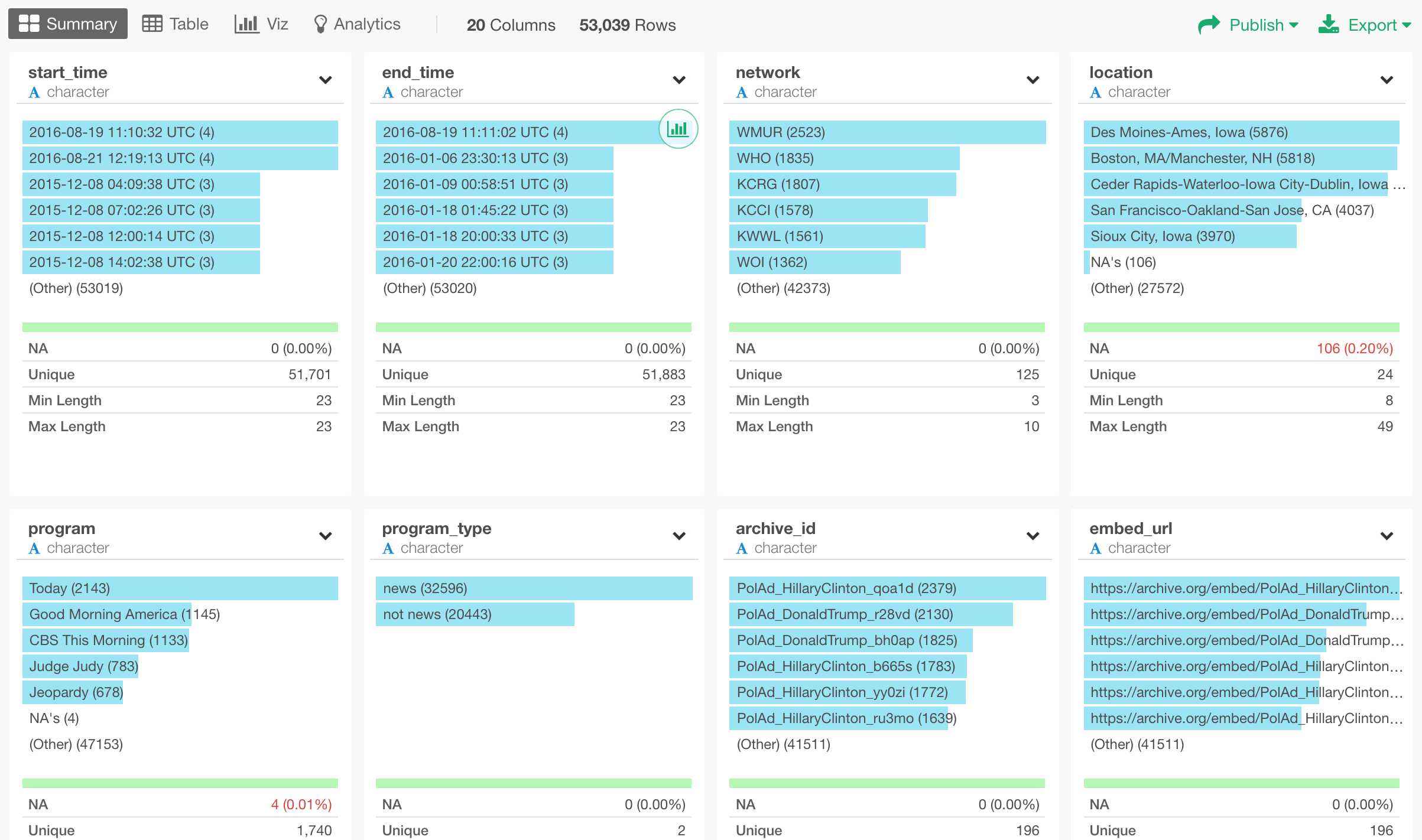
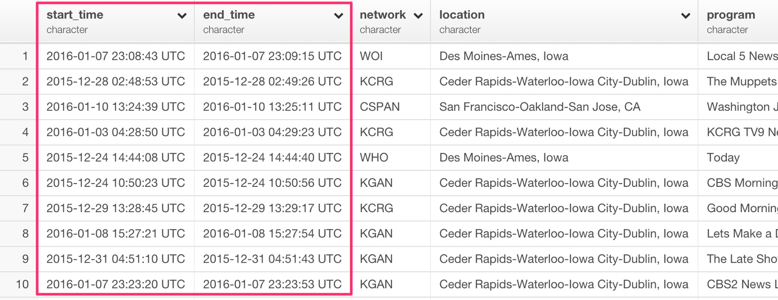
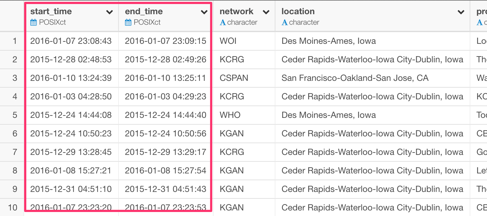
There are two columns called ‘start_time’ and ‘end_time’, which indicate what time each of the TV ads started and ended.
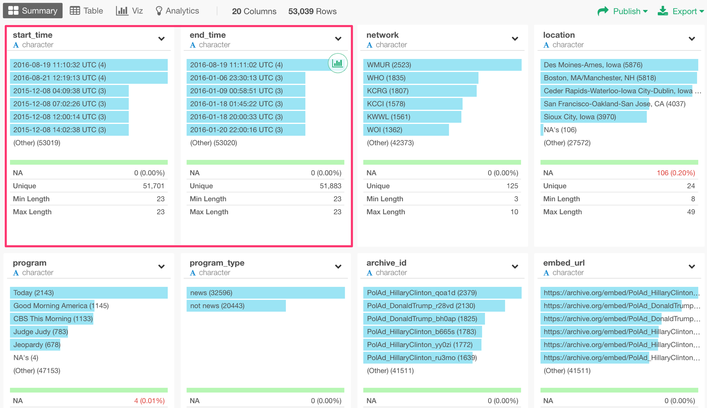
The problem is that these twese two columns came in as Character data type.
To make the analysis easier later, we want to convert these to Date/Time data type. This data contains both Date and Time so we want to convert them as POSIXct data type.
You can select ‘Change Data Type’ -> ‘Convert to Date / Time’ from the column header menu.

Since the data is in an order of ‘Year, Month, Day, Hour, Minute, Second’, you want to select ‘Year, Month, Day, Hour, Minute, Second’ from the sub-menu.
This will create a ‘mutate’ step with an expression like below.
ymd_hms(start_time)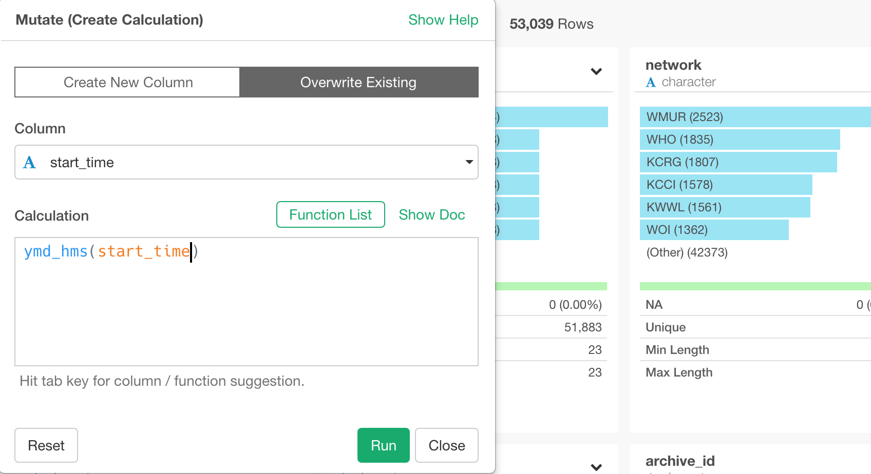
This ‘ymd_hms’ function stands for:
- y - Year
- m - Month
- d - Day
- h - Hour
- m - Minute
- s - Second
It can be used for any text / numeric data that follows ‘Year, Month, Day, Hour, Minute, Second’ order.
Anyway, once you run the above step, you will get the ‘start_time’ column converted to POSIXct data type and the Summary view shows a nice histogram showing the range of the data.
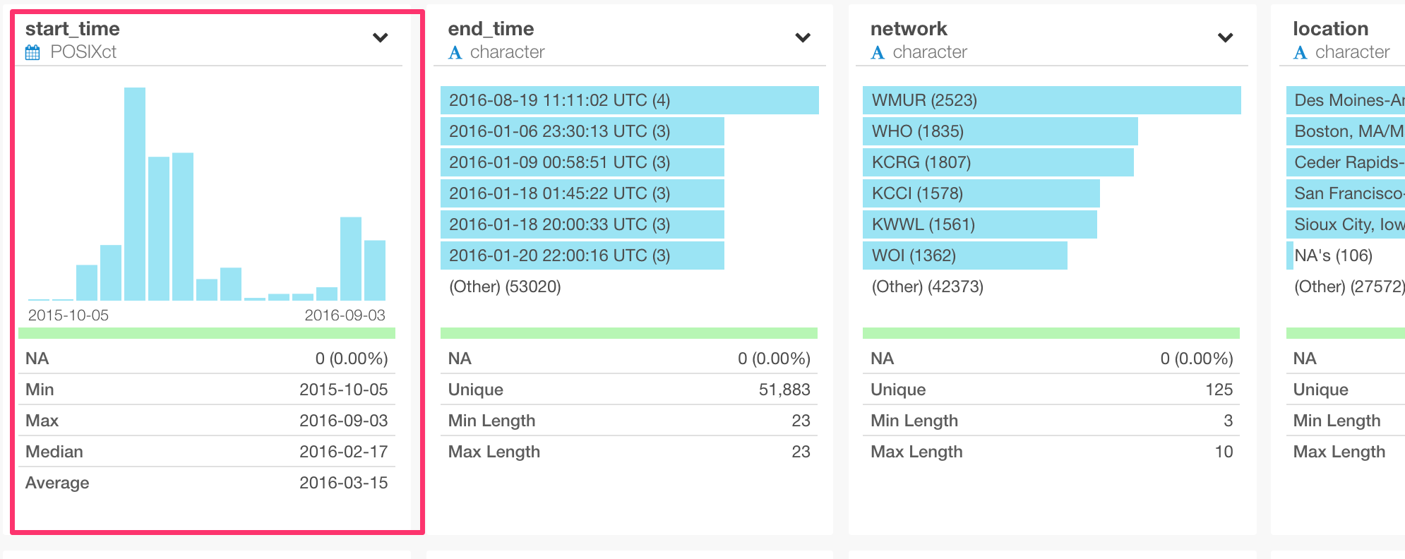
Now, you can do all sorts of things with this data.
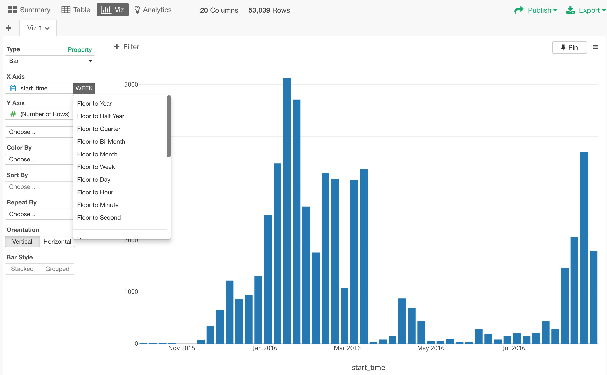
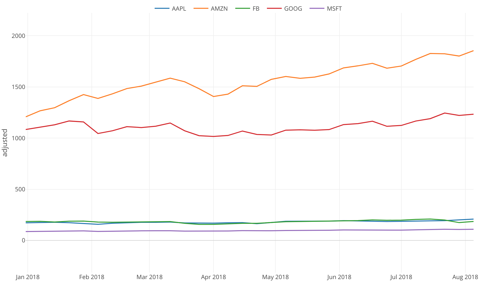
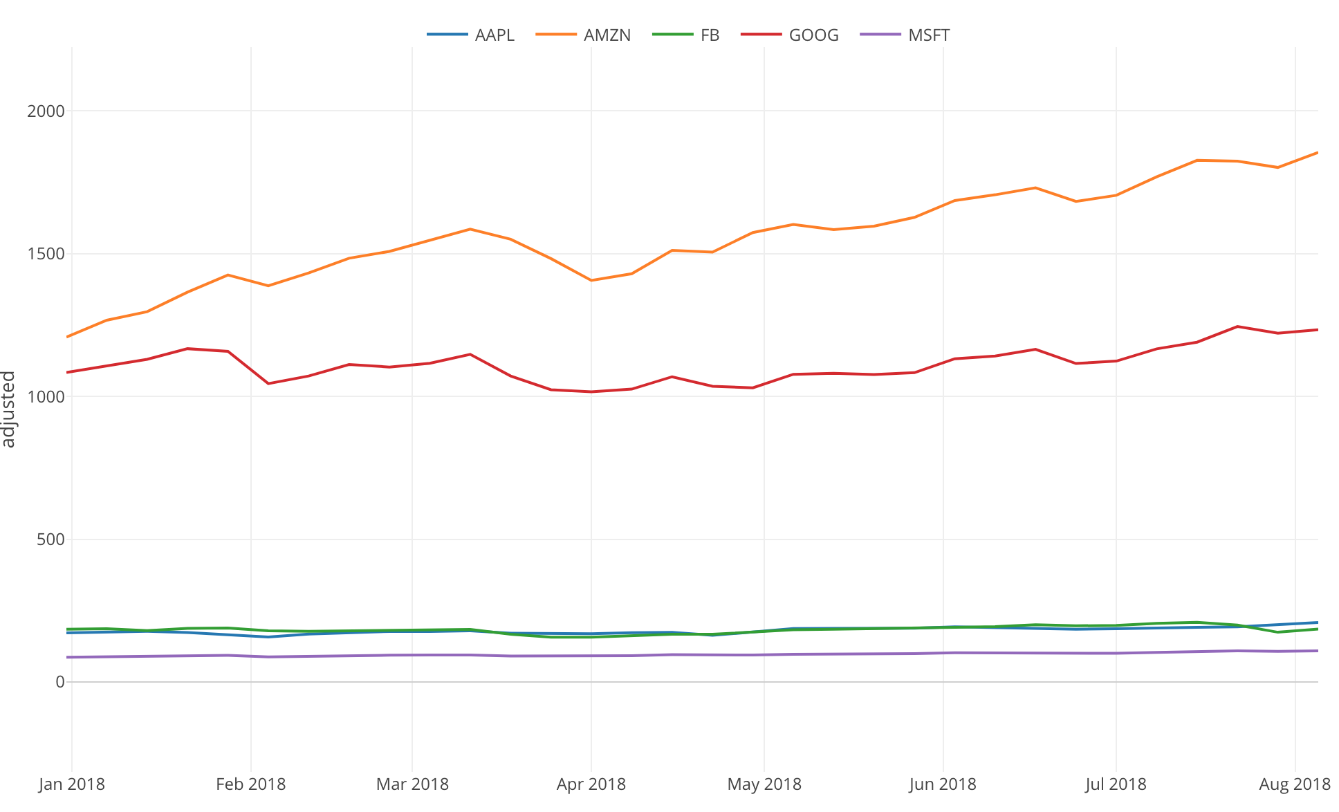
For example, you can go to Chart view, assign these new columns to X-Axis, and switch the aggregation level to something like Year, Month, Quarter, Week, etc.
Other Date / Time Formats
What if you have only Year, Month, and Day, but not Time part of the data?
Then, there is a function called ‘ymd’.
Ok, then what if the date and time data doesn’t come in ymd_hms format?
For example, you might get data like below.
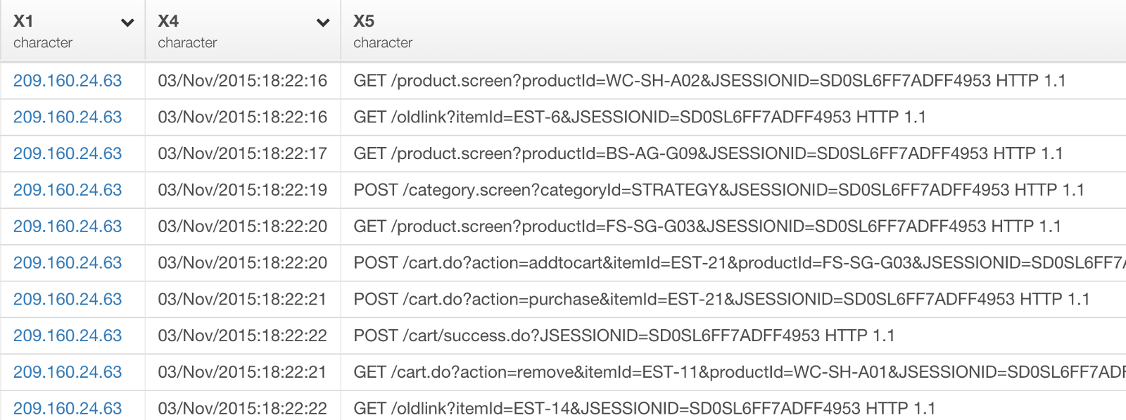
The X4 column has the characters ordered in Day, Month, Year, Hour, Minute, and Second.
Well, there is a function called dmy_hms that is literally reflecting the order of the data.
These functions are all coming from an R package called ‘lubridate’ and they are super powerful.
It doesn’t matter what characters are between the date and time attributes like Year, Month, Day, etc. For example, ymd function can take any of the following data and convert them to Date type appropriately.
2018-04-02

2018/04/02

2018/4/2

Reported on 2018, April 2nd.
What it matter is the order in which Year, Month, and Day are presetented.
It just works.
Non English Locale?
What happens if the month names came in as different languages other than English? Well, you can simply set the locale like below and that will parse the characters appropriately.
ymd_hms(start_time,locale="ja_JP")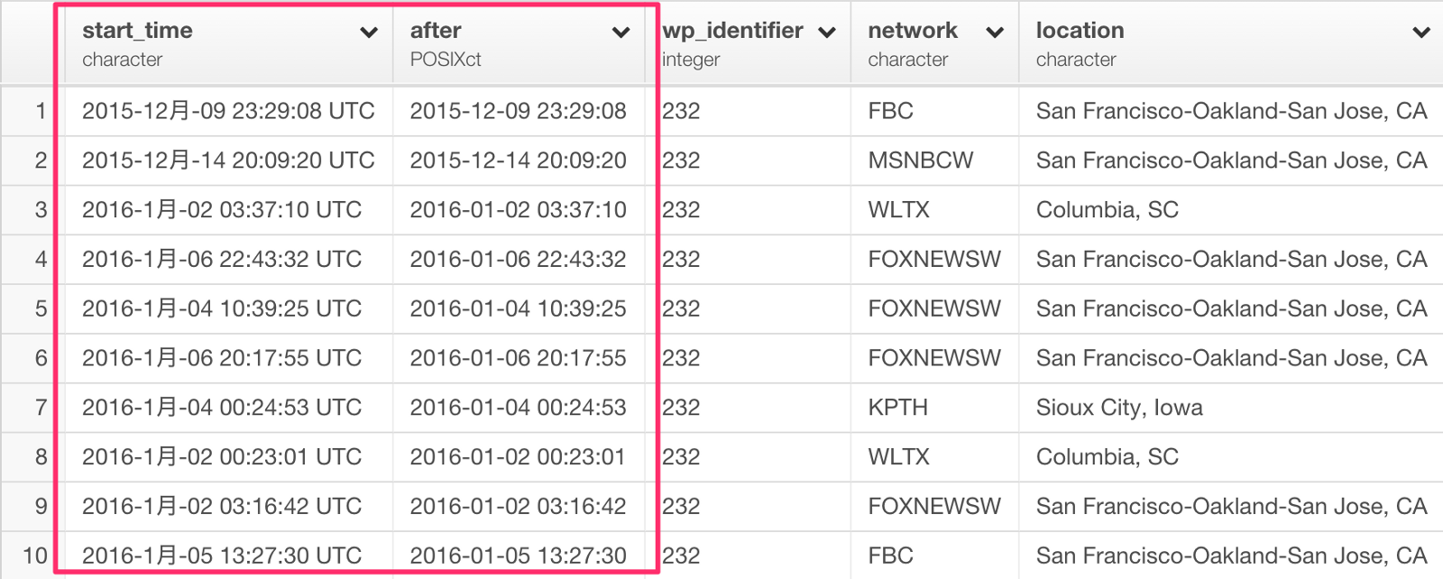
Handling Timezone
Did you notice that the original data had “UTC” as the timezone information in the text?
This means that the ‘ymd_hms’ function takes this timezone information into account when converting to POSIXct. But many of us don’t live in UTC timezone, and we usually want the time to be shown in our local timezone.
Well, there is a function called ‘with_tz’ to take care of just that.
with_tz(start_time)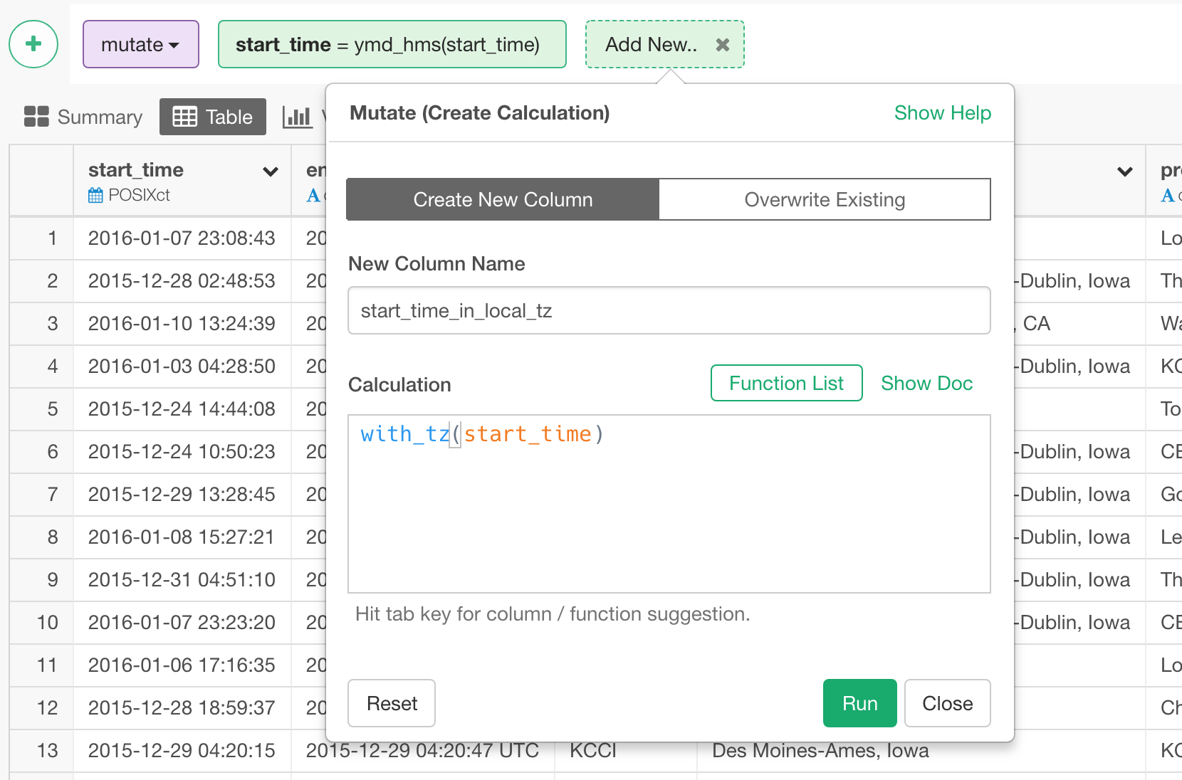
Now, you can compare the original time (UTC) and the converted time in your local timezone. (It’s Pacific Timezone in the picture below because I run this in San Francisco, California.)
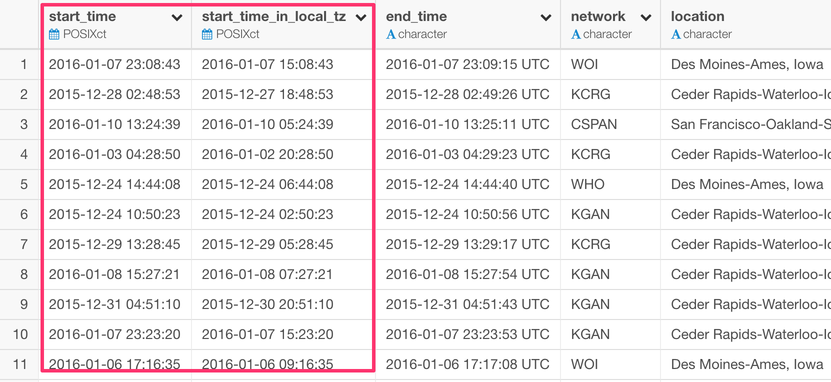
with_tz function takes the system default timezone of your PC, but in case you want to set a particular timezone, let’s say, East Coast (US) time, you can use ‘tz’ argument like below.
with_tz(start_time, tz = "America/New_York")2. Extract Values from Date / Time Data
Sometimes you want to compare data by Month names like January, February, or Day of Week like Sunday, Monday, etc.
There is a comprehensive set of functions from ‘lubridate’ package you can use to get this job done easily. I’m going to introduce just a few here.
Extracting Month Name
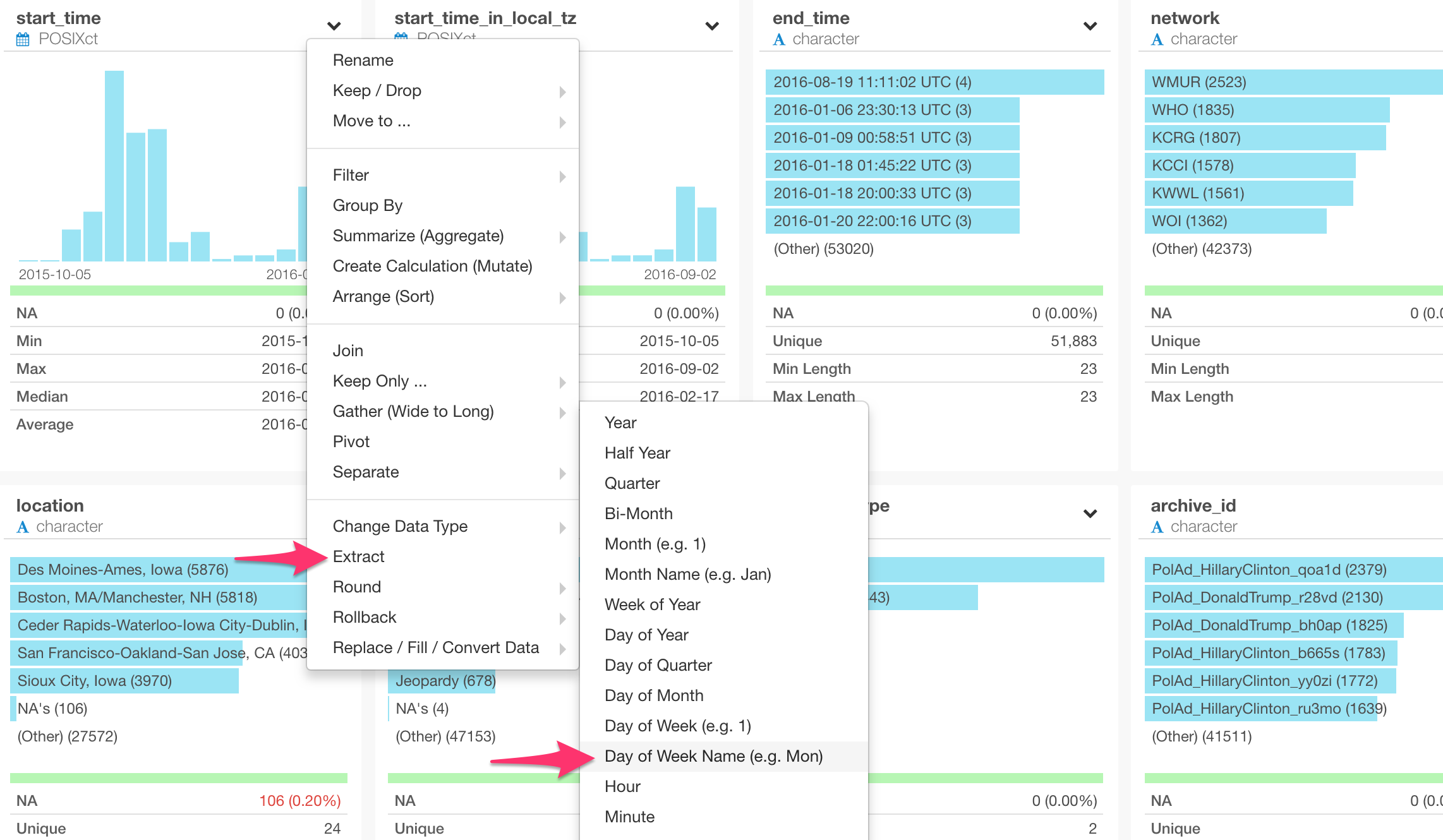
Let’s start from extracting the month names.
Select ‘Extract’ -> ‘Month Name’ from the column header menu.
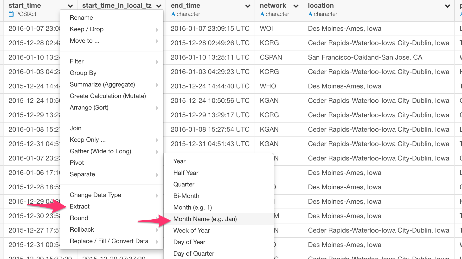
This will populate month function like the below.
month(start_time, label = TRUE, abbr = TRUE)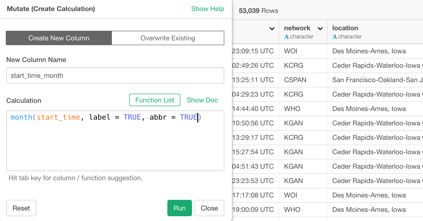
month function extracts the month information from Date & Time data. You can use ‘label’ argument to decide whether you want it to return something like “Jan”, “Feb”, “March”, etc. or 1, 2, 3. etc.
The cool thing about this is that it returns the values as ‘Ordered Factor’, which means it has the order (sorting) information embedded in the data. Therefore, when you sort or summarize data in R it would respect the pre-defined order and return the values the way you would expect.
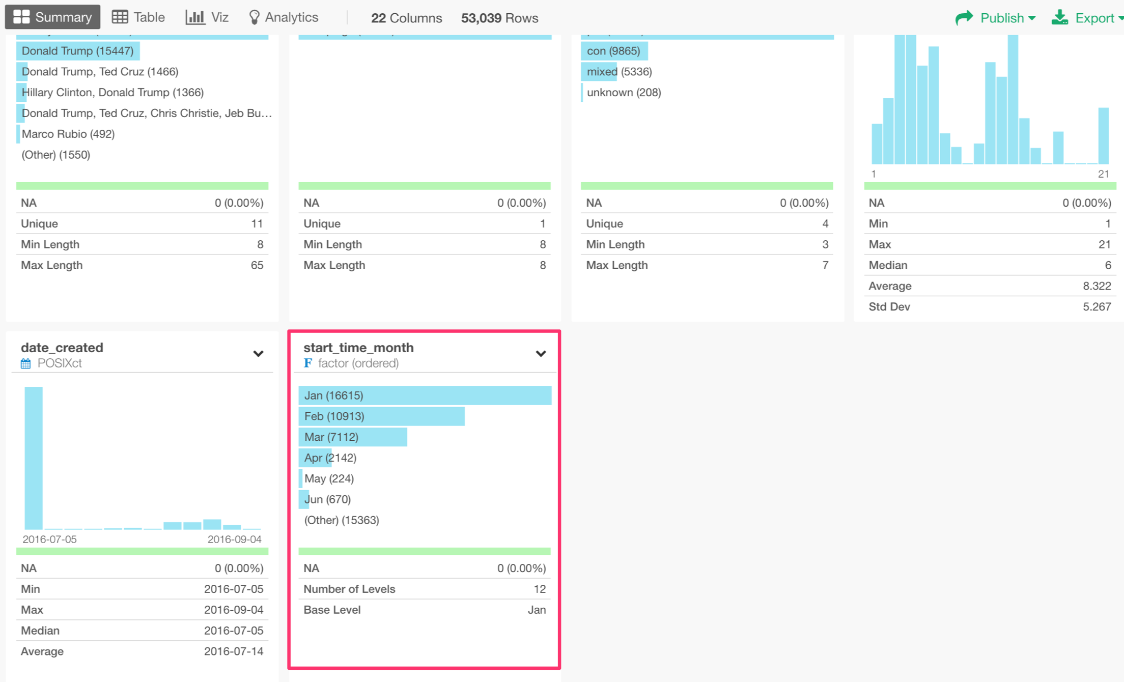
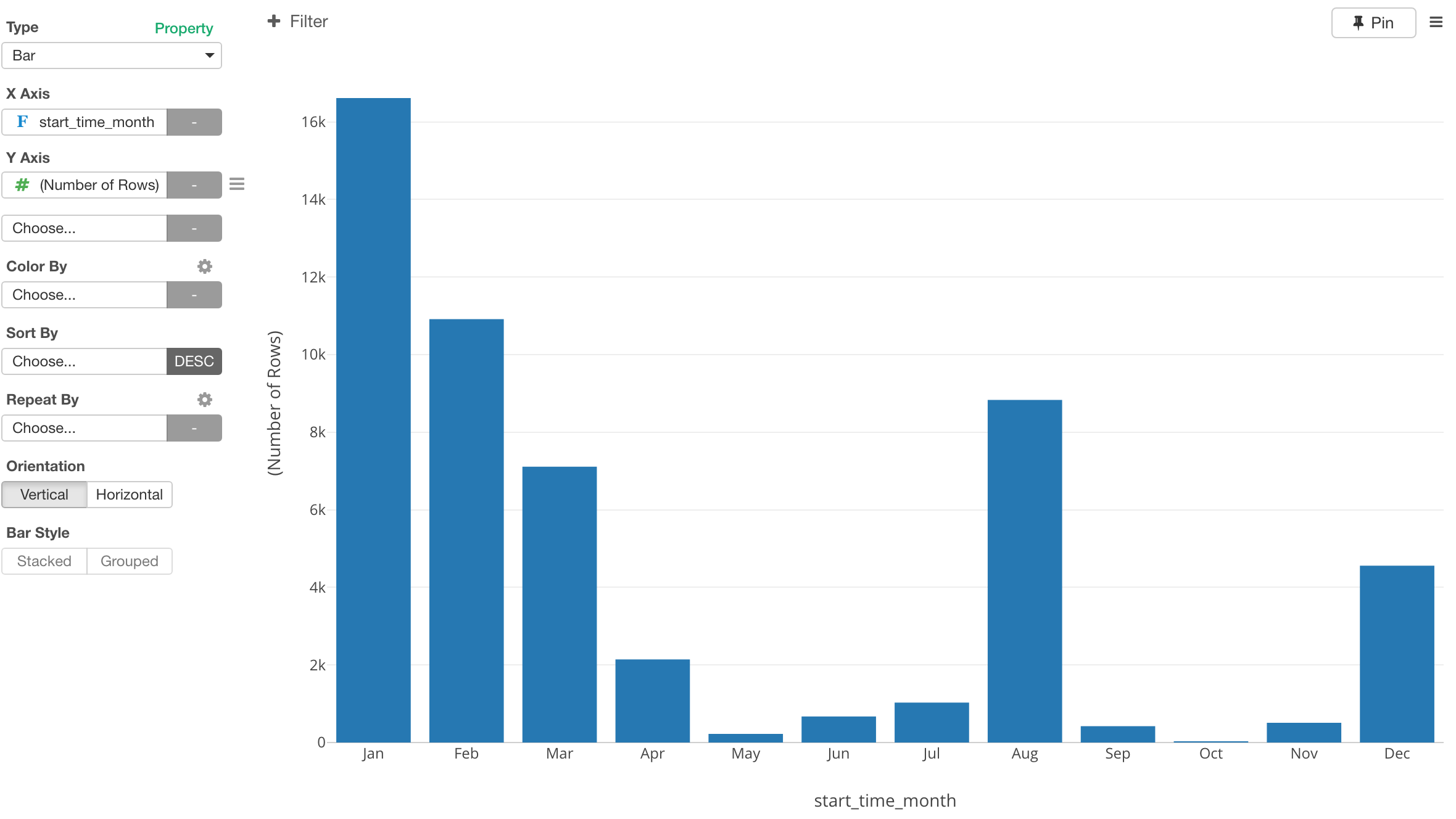
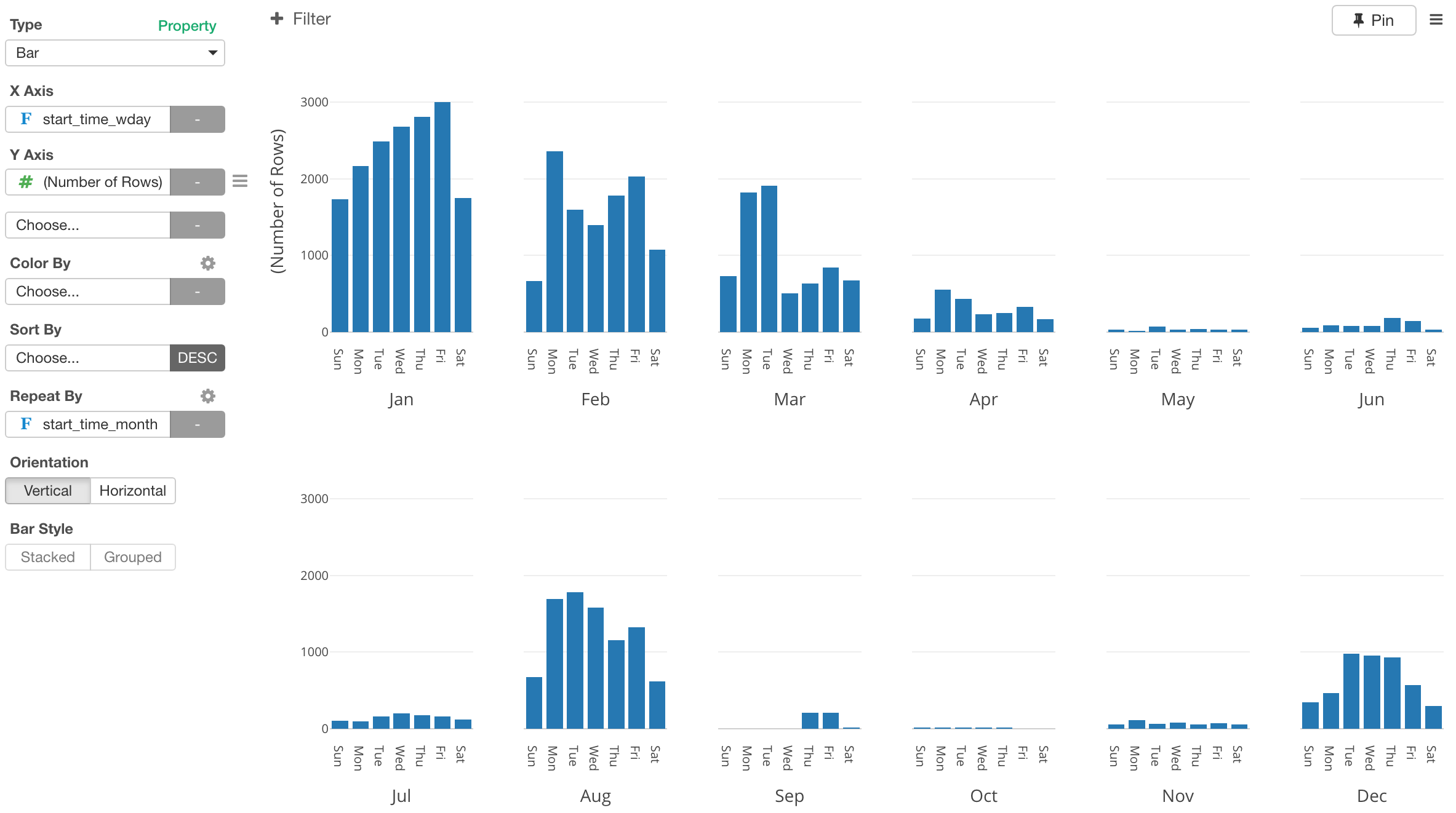
You can try to see this with any charts.
Month Name in Bar Chart
Extracting Day of Week
Second, let’s extract the day of week.
Select ‘Extract’ -> ‘Day of Week’ from the column header menu.
This will populate wday function like the following.
wday(start_time, label = TRUE, abbr = TRUE)You can use ‘label’ argument to decide whether you want it to return something like ‘Sun’, ‘Mon’, ‘Tue’, etc. or 1, 2, 3, etc.
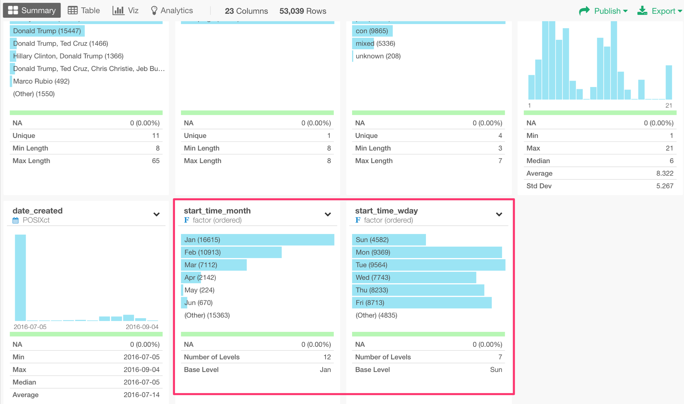
This wday function also returns the values as ‘Ordered Factor’. This means, when you summarize or sort the data, it will appropriately return the data in an order that you would expect, like below.
3. Filter based on Date and Time
Sometimes we want to filter the data based on date and time information.
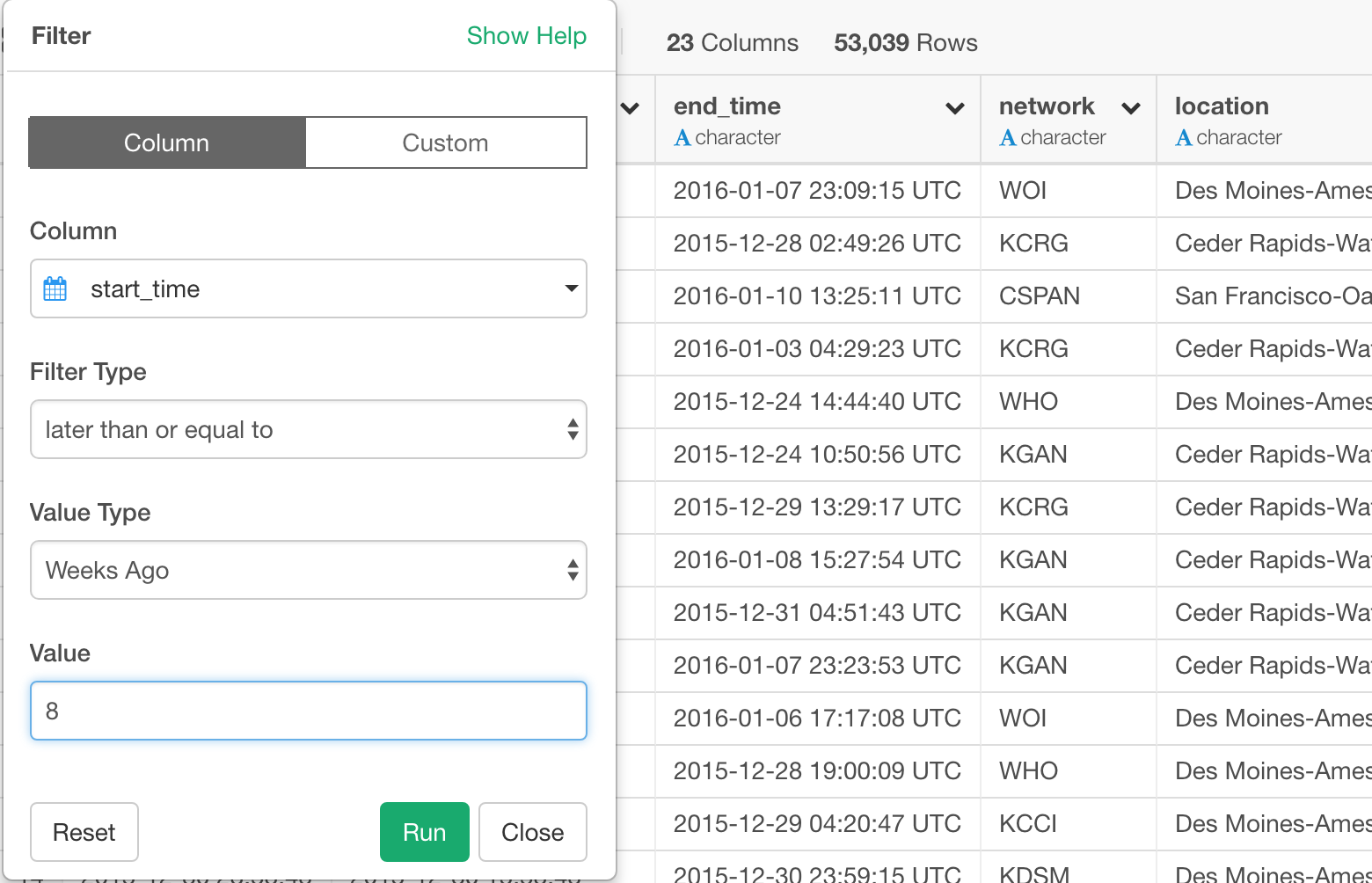
Let’s say we are interested in the data for the last 8 weeks.
Select ‘Filter’ -> ‘later than or equal to’ -> ‘Weeks Ago’ from the column header menu.
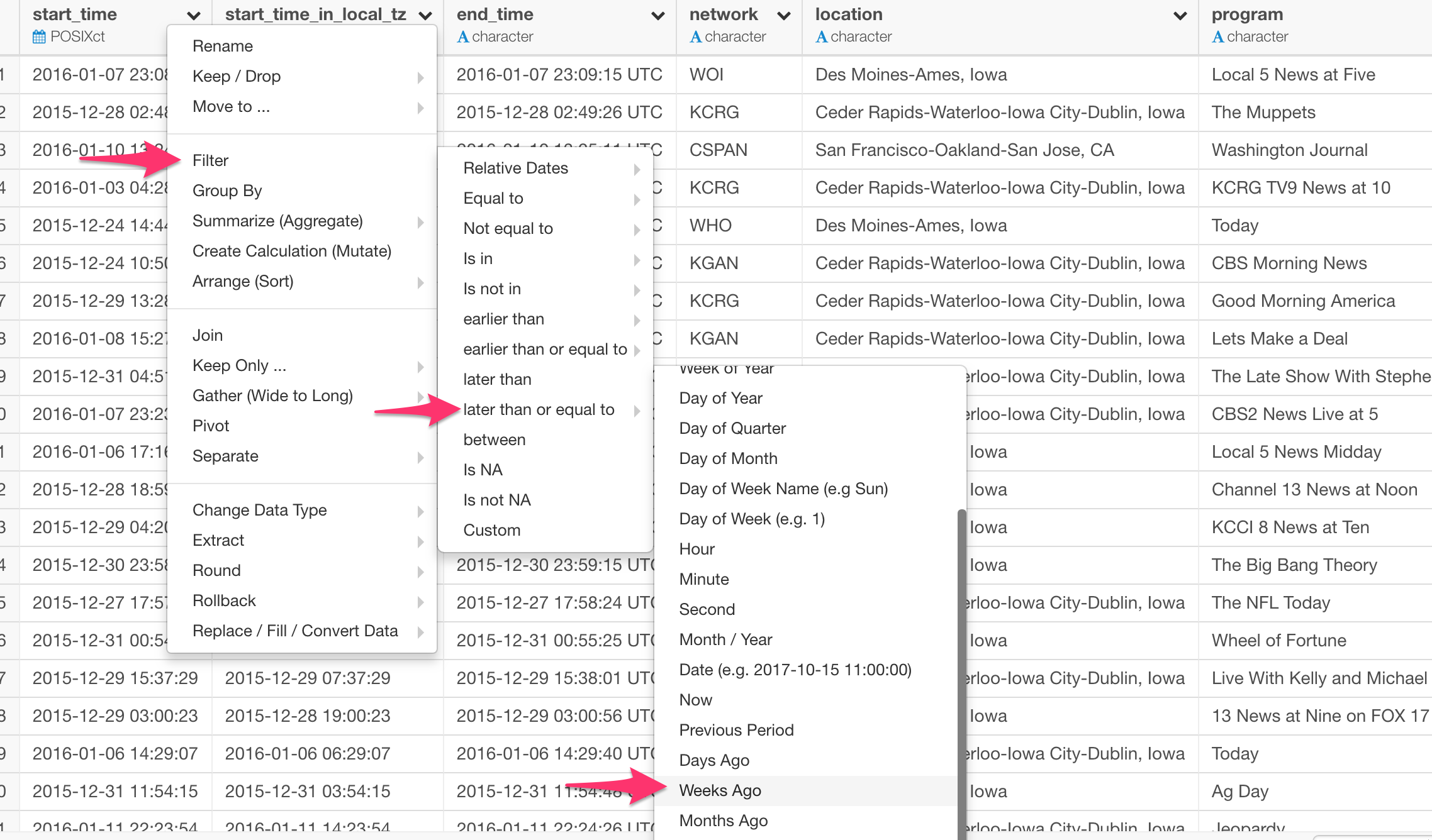
And type 8 for the Value.
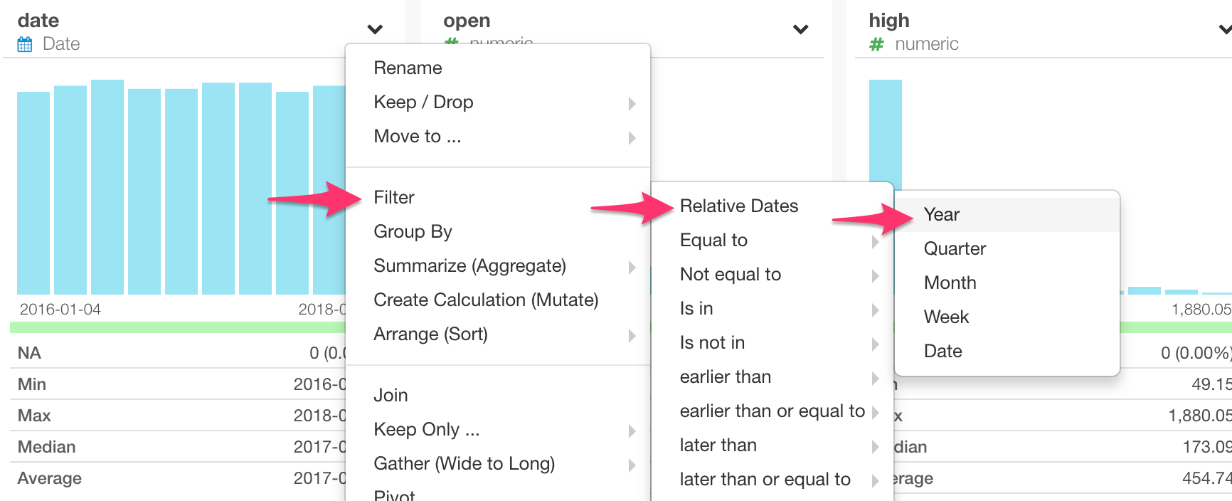
Filter with Relative Dates
There is a list of Relative Dates types for filtering data.
- Previous Year
- This Year
- Next Year
- Last N Years
- Year to Date
Let’s take a look at the difference among some of them.
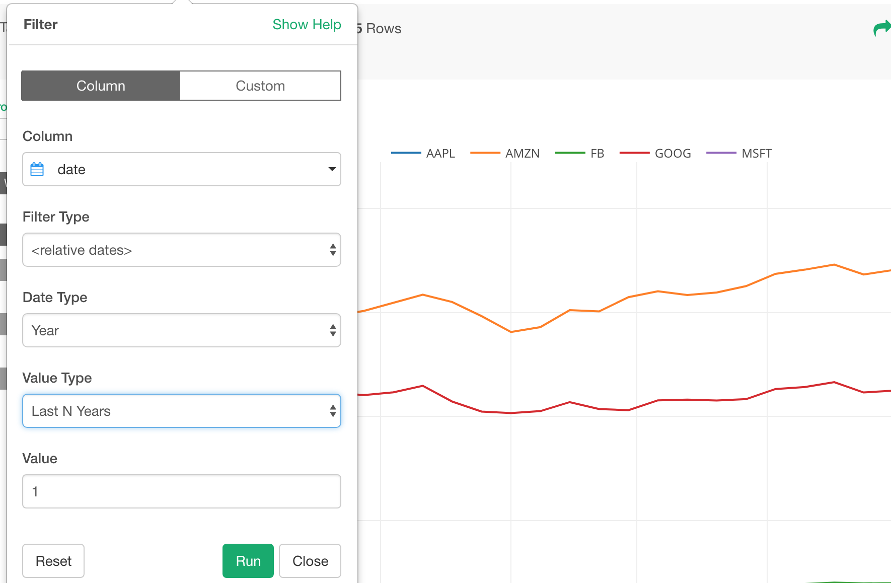
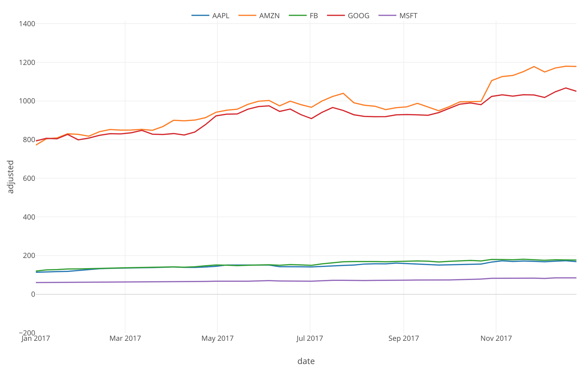
Last N Years
This will return the data starting January and ending December of the last N year(s). Here’s an example ‘Last 1 Year’.
Previous (Last) Year
Previous Year returns the data from January to December of the last year.
This Year
This Year returns the data from January to December of this year. The sample data below had only up to August (as of writing), this is why it’s showing from January to August.
Year to Date
Year to Date returns the data starting from January of the current year (January) to today.
4. Calculate the length between two date and times
Let’s say we want to calculate how long each TV commercial was running for.
Select ’Create Calculation (Mutate) from the column header menu.
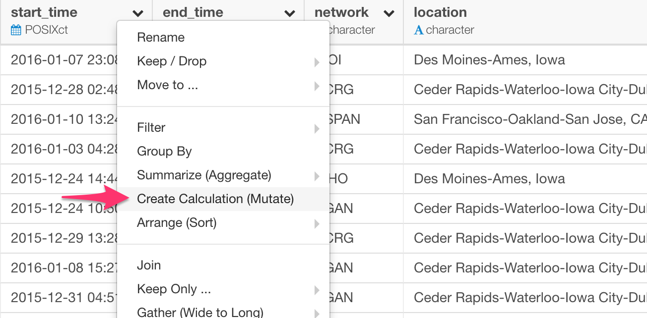
We can simply use ‘-’ to subtract ‘start_time’ from ‘end_time’ like below.
end_time - start_time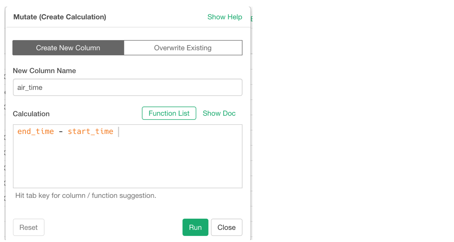
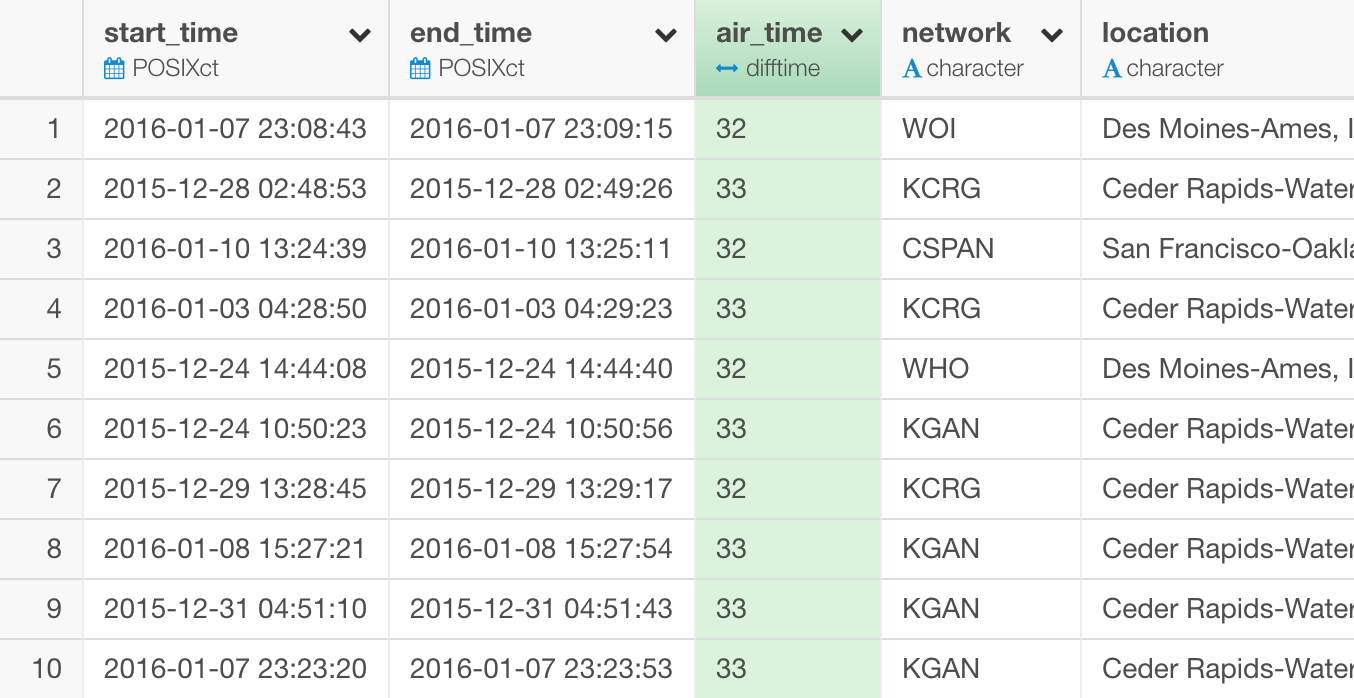
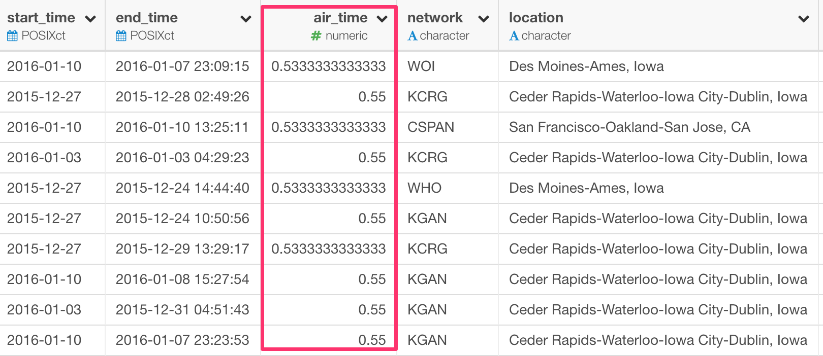
This will create a new column as ‘difftime’ data type, which is a special data type in R that holds the date/time duration information. The unit is seconds for the calculations with POSIXct data type and days for the calculations with Date data type.
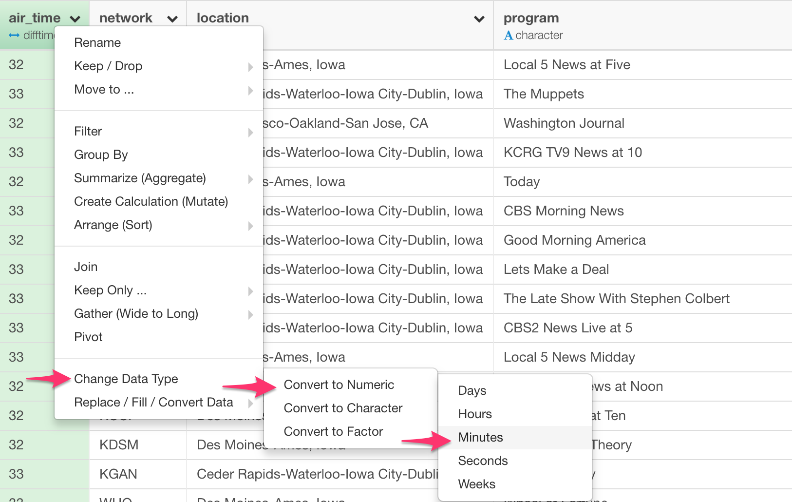
In most cases though, we want to see the values presented as Numeric data type, which makes all the calculations easier later.
Select ‘Change Data Type’ -> ‘Convert to Numeric’ -> ‘Minutes’ if you want to convert it to Numeric data with Minutes as the unit.
This will populate as.numeric function and you can customize it like the below.
as.numeric(end_time - start_time, units="mins")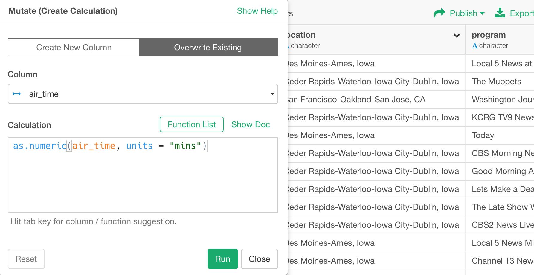
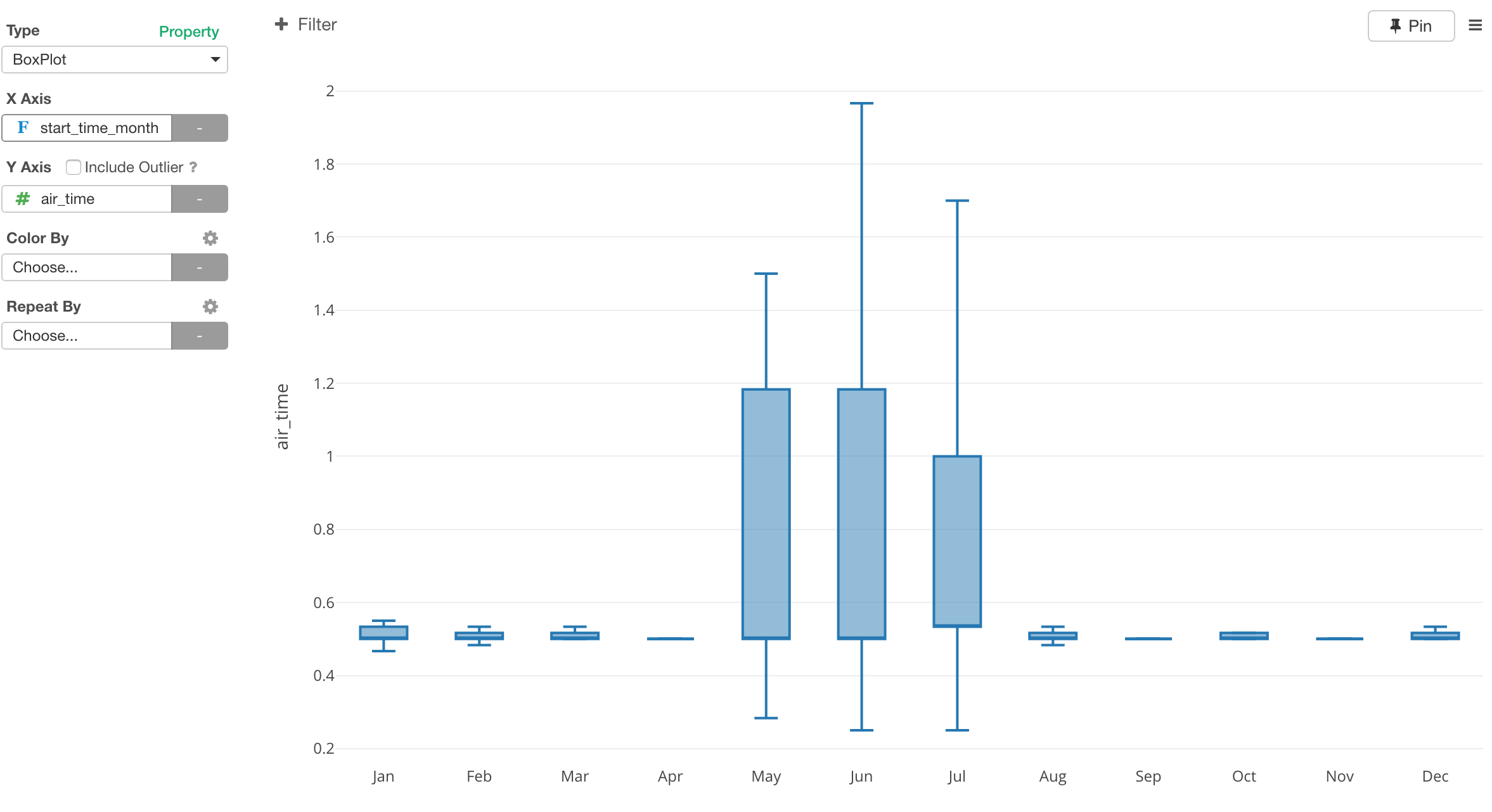
We can visualize this data to see which months run longer or shorter TV commercials.
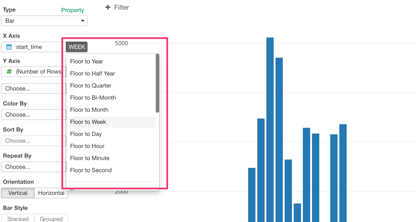
5. Round Date & Time Values
Sometimes, you want to round date values to a certain level like month, week, day, etc, so that you can aggregate data by that level.
Select ‘Round’ -> ‘Round Date’ -> ‘Week’ from the column header menu if you want to round it to the Week level..
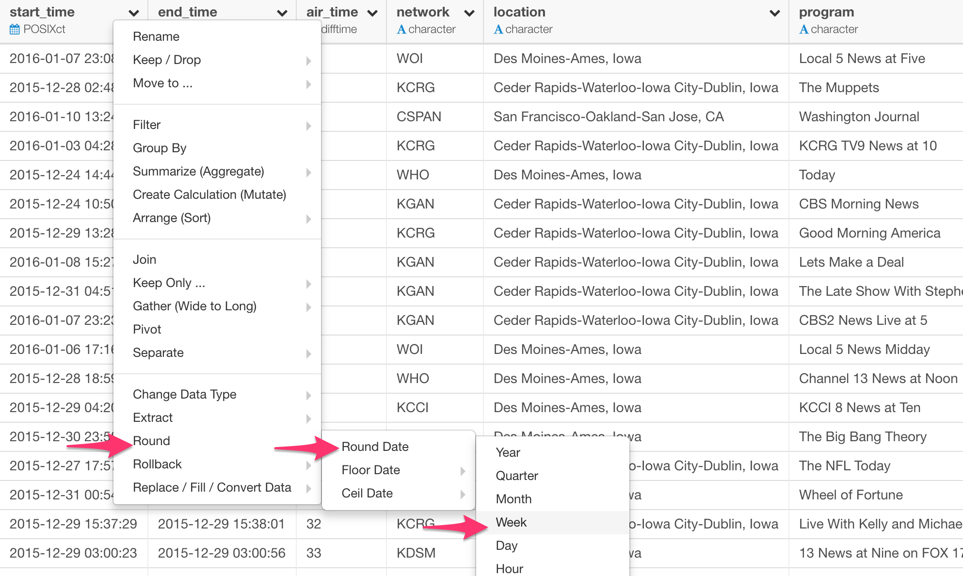
This will populate ‘round_date’ function like below.
round_date(start_time, unit="week")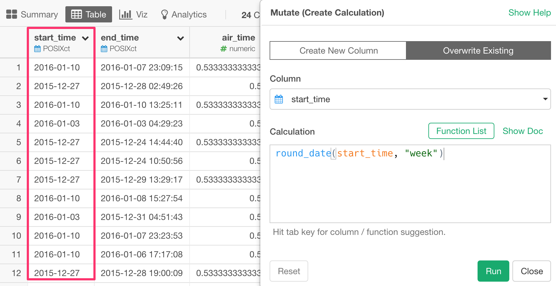
There are ceiling_date to round up and floor_date to round down the date and time values as well.
floor_date(start_time, unit="week")In Exploratory, in most cases you actually don’t need to do this manually.
Instead, you can simply use one of the chart types to get the same result by switching the aggregation levels like the below! 😉