How to Collect Unemployment Data for all the California Counties from FRED
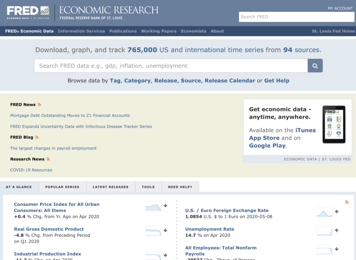
FRB (Federal Reserve Bank) collects tons of economic data (765,000!) such as Unemployment Rate, GDP, Treasury Rate, etc. and amazingly, it publishes the data on their website called FRED (Federal Reserve Bank Economic Data) for public access.
As I have shown in another post 'How to Collect Unemployment Data for all the US States from FRED', you can write a custom R script to import the data directly from FRED in Exploratory.
In this post, I'm going to show you how to collect the unemployment data for all the California Counties.
Collect Data for All California Counties
It turned out we can collect the unemployment rate data at the US County level as well.
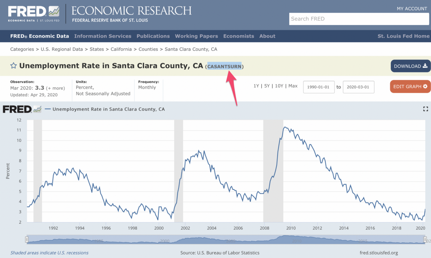
Let’s say we want to collect the data for Santa Clara County in California. (this is where many of the Silicon Valley companies like Apple, Google, Netflix, etc.) are located.
Here is the page for the unemployment rate in Santa Clara County.
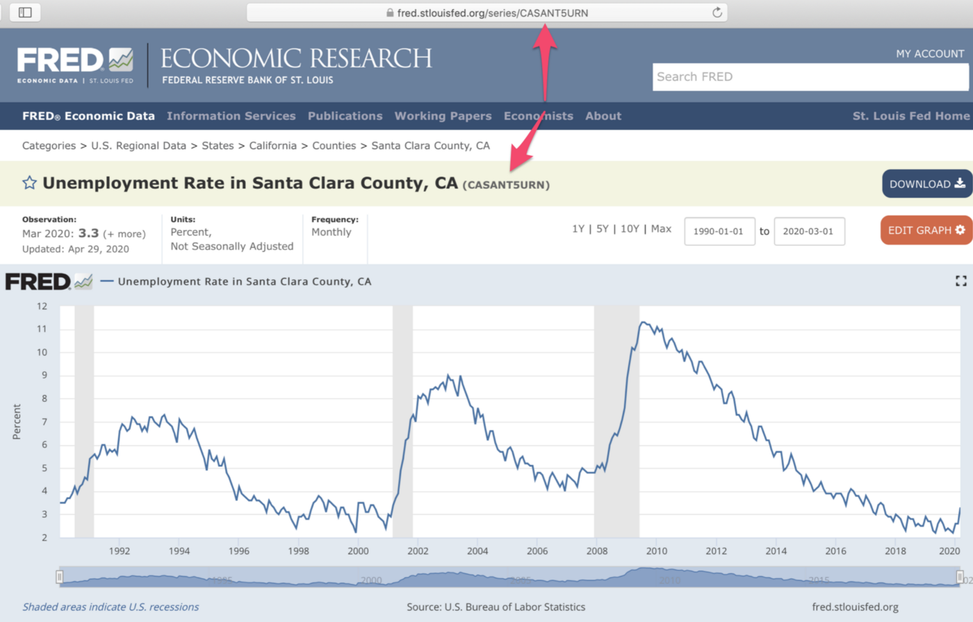
Basically, the same thing. You want to copy the code for this data then use the same ‘tq_get’ function.
library(tidyquant)
tq_get("CASANT5URN", get = "economic.data", from = "1999-01-01")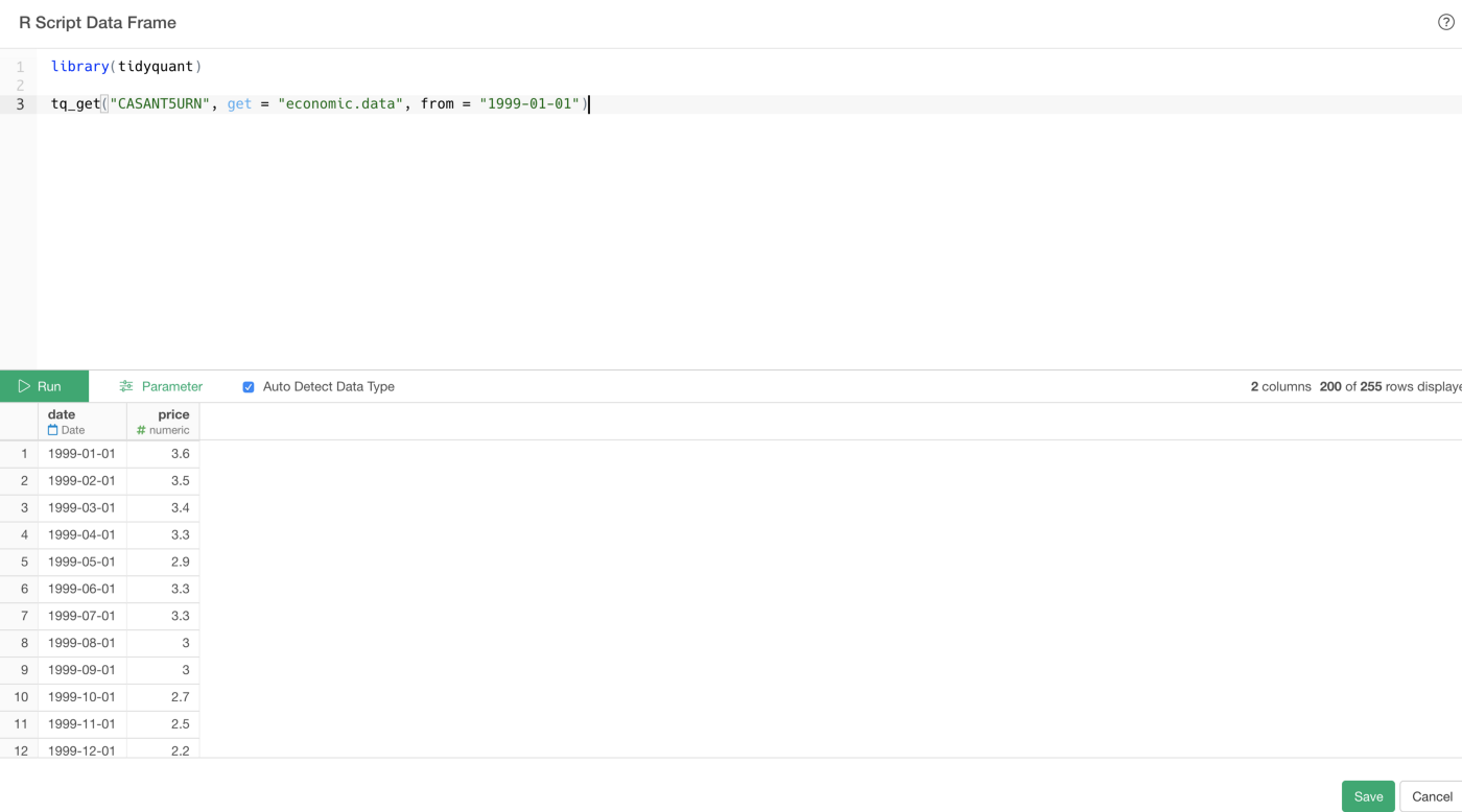
Now, we have 58 counties in California, how can we get the unemployment rate data for all of them?
We can do pretty much the same thing as we did for the US States, except that constructing a list of the county codes is a bit tricky.
This page lists up all the California Counties. You can click each of the Counties and open the unemployment rate page. But the county code part is a bit weird.
Here’s one for Santa Clara.
And here’s one for San Mateo.

To this day, I still can’t figure out how they came up with those county codes and I haven’t found the list yet.
So I’ve created the list by myself! Yes, manually, one by one, for California counties and published it here.
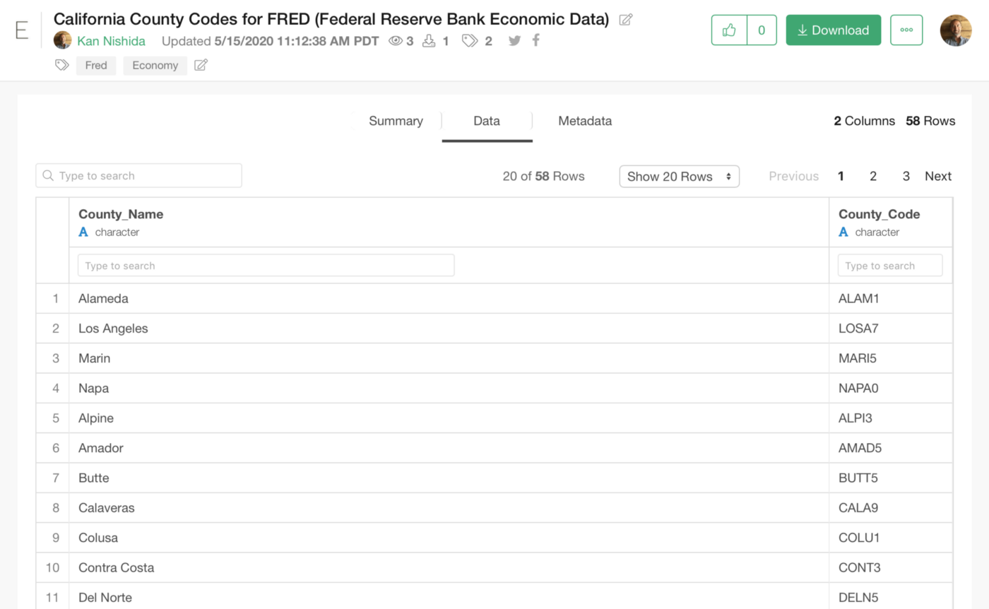
And this data can be accessed via REST API (HTTPS).
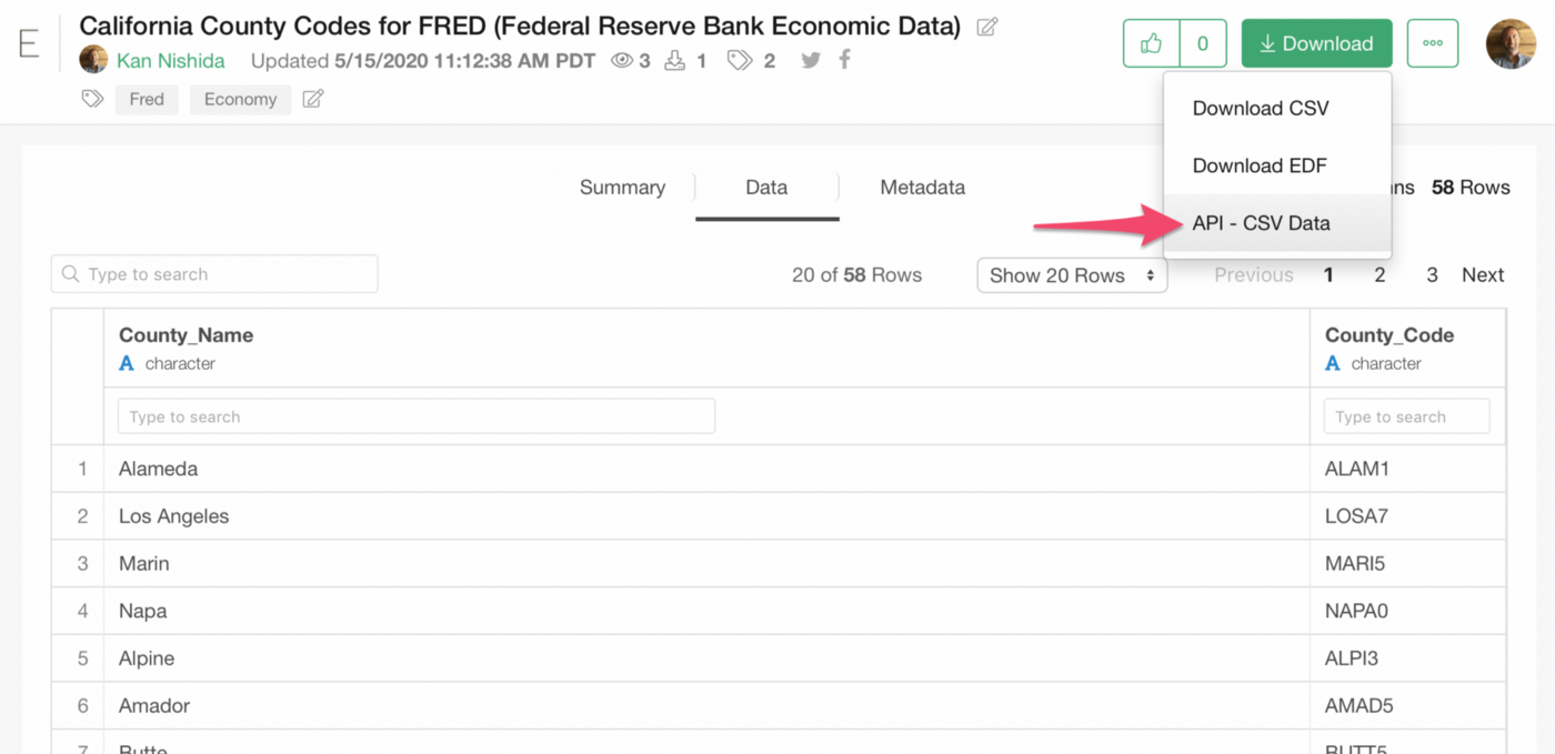
as an URL like the below.
https://exploratory.io/public/api/kanaugust/California-County-Codes-for-FRED-Federal-Reserve-Bank-Economic-Data-thi1rkw0ky/data?api_key=EyT6bdF8CamrN5yKD4IYGKd2Dam7QASo, by using the above data, we can write something like below.
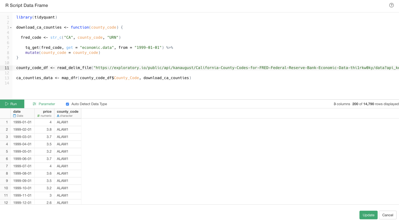
library(tidyquant)

county_code_df <- read_delim_file("https://exploratory.io/public/api/kanaugust/California-County-Codes-for-FRED-Federal-Reserve-Bank-Economic-Data-thi1rkw0ky/data?api_key=EyT6bdF8CamrN5yKD4IYGKd2Dam7QA", ",")

download_ca_counties <- function(county_code) {

  fred_code <- str_c("CA", county_code, "URN")

  tq_get(fred_code, get = "economic.data", from = "1999-01-01") %>%
  mutate(county_code = county_code)
}

ca_counties_data <- map_dfr(county_code_df$County_Code, download_ca_counties)
It might look complicated, but it’s relatively straightforward.
First, the ‘read_delim_file’ function imports the above URL data, the one I have published to the Exploratory Data Catalog, and the data get stored in the ‘county_code_df’ data frame.
Then, I’m registering a function called ‘download_ca_counties’, which does pretty much the same thing as the one for the States.
It performs:
- Construct the FRED code (e.g. CASANT5URN) with the ‘str_c’ function.
- Call the ‘tq_get’ function and pass the FRED code.
- Call the ‘mutate’ command to create a new column ‘county_code’ with the value of the ‘county_code’ variable.
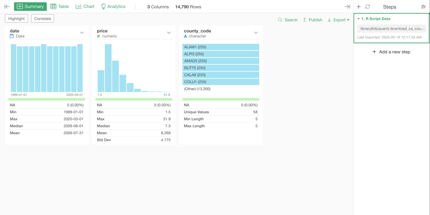
Finally, the ‘map_dfr’ function runs the ‘download_ca_counties’ function as many times as a number of values in the ‘County_Code’ column of the ‘county_code_df’ data frame, which is 58 by the way.
And when you copy and paste the above code and run it you would get a data frame with 3 columns, date, ‘price’, which has the unemployment rate, and ‘county_code’.
We can click on the ‘Save’ (for the first time) or the ‘Update’ (after the second time) button to import the data into Exploratory.
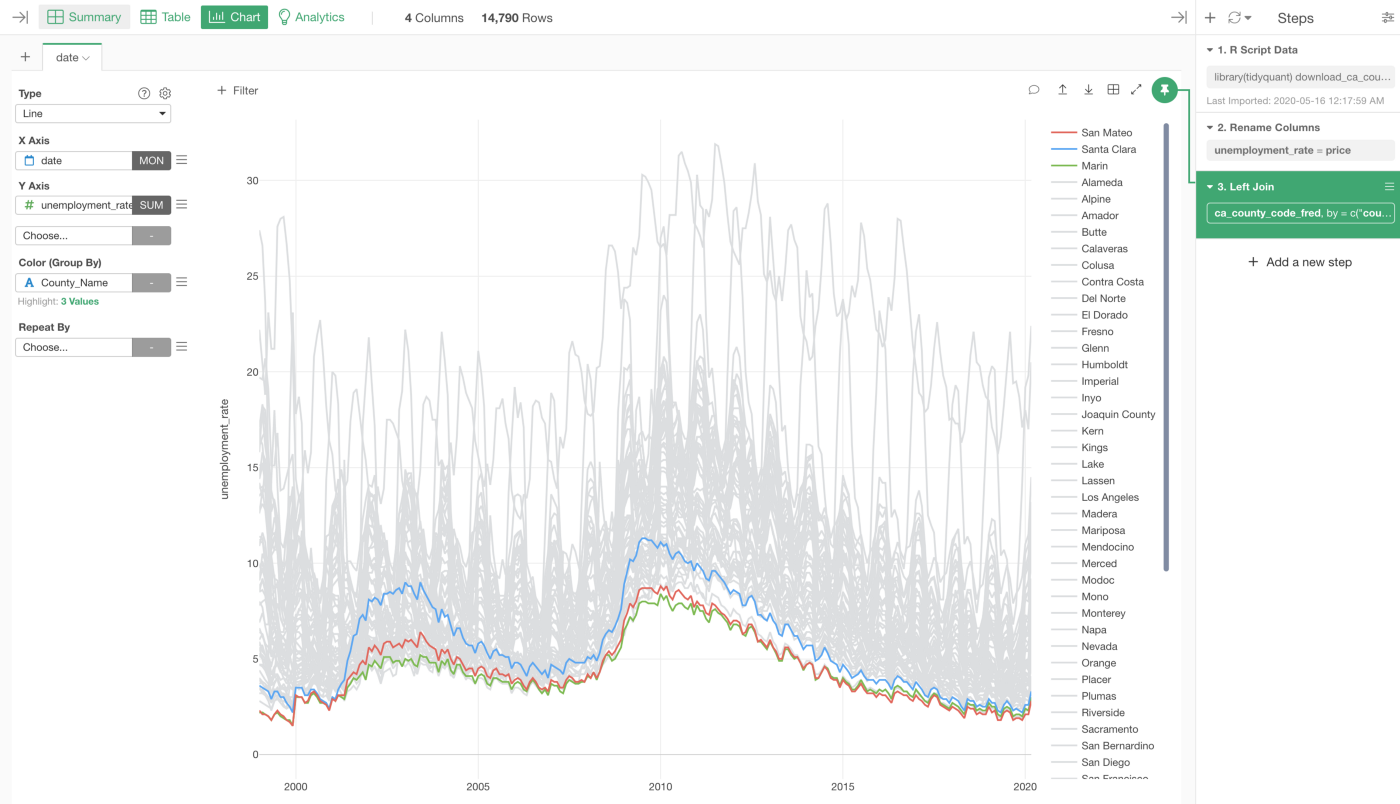
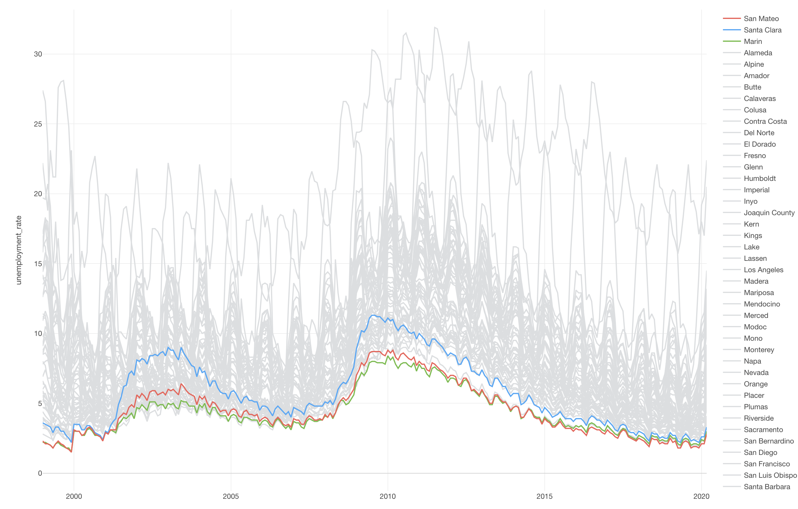
And we can rename the ‘price’ column name as we did before. I’ll skip the part for now. And finally, we can visualize the data under the Chart view.