How to Create Table 1 Summary Information
Table 1 is a common format to show summary statistics of data that is used in medical research papers.
You can use a various data wrangling mehods such as Group By, Summarize, etc. to calculate such statistics.
But, in R, there is a package called ‘tableone’, which is designed to generate the Table 1 information.
This means, you can quickly use the package to generate Table 1 information in Exploratory.
There are two ways to use this package.
One way is to use Note, which is based on RMarkdown, where you can directly write R script with the ‘tableone’ package and produce the result as output. This is a simple and quick solution if you are ok with the output in Note.
Another is to create a custom R function with the ‘tableone’ package and call it as a data wrangling step. This would take a bit of steps, but since you will get the result in a data frame format you will be able to use the data in a more flexible way.
Sample Data
If you’re interested, you can download a sample data for this exercise from this link.
tableone R Package Install
You can install the ‘tableone’ R package inside Exploratory.
A. Use Note
Here is an R script
library(tableone)

# Create a variable list which we want in Table 1
listVars <- c("Age", "Gender", "Cholesterol", "SystolicBP", "BMI", "Smoking", "Education")

# Define categorical variables
catVars <- c("Gender","Smoking","Education")

table1 <- CreateTableOne(vars = listVars, data = table_one_copy_1, factorVars = catVars, strata = c("Gender"))


a <- print(table1, quote = TRUE, noSpaces = TRUE)

as.data.frame(a)
And you want to have this script inside of R script area.
Click on ‘R Code’ button in the toolbar.
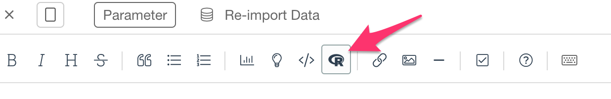
Then, copy and paste the above script inside the R Script area.
When you run it, you will see the following output inside Note.
##                            "Stratified by Gender"
##  ""                         "Female"         "Male"           "p"
##   "n"                       "143"            "107"            ""
##   "Age (mean (sd))"         "56.94 (8.05)"   "58.25 (7.55)"   "0.191"
##   "Gender = Male (%)"       "0 (0.0)"        "107 (100.0)"    "<0.001"
##   "Cholesterol (mean (sd))" "224.80 (25.06)" "223.21 (24.78)" "0.620"
##   "SystolicBP (mean (sd))"  "144.95 (10.99)" "146.27 (8.71)"  "0.305"
##   "BMI (mean (sd))"         "26.74 (4.58)"   "26.84 (4.09)"   "0.859"
##   "Smoking = Yes (%)"       "37 (25.9)"      "35 (32.7)"      "0.298"
##   "Education (%)"           ""               ""               "0.289"
##   "   High"                 "56 (39.2)"      "52 (48.6)"      ""
##   "   Low"                  "45 (31.5)"      "26 (24.3)"      ""
##   "   Medium"               "42 (29.4)"      "29 (27.1)"      ""
##                            "Stratified by Gender"
##  ""                         "test"
##   "n"                       ""
##   "Age (mean (sd))"         ""
##   "Gender = Male (%)"       ""
##   "Cholesterol (mean (sd))" ""
##   "SystolicBP (mean (sd))"  ""
##   "BMI (mean (sd))"         ""
##   "Smoking = Yes (%)"       ""
##   "Education (%)"           ""
##   "   High"                 ""
##   "   Low"                  ""
## " Medium" ""| “Female” | “Male” | “p” | “test” | |
|---|---|---|---|---|
| “n” | 143 | 107 | ||
| “Age (mean (sd))” | 56.94 (8.05) | 58.25 (7.55) | 0.191 | |
| “Gender = Male (%)” | 0 (0.0) | 107 (100.0) | <0.001 | |
| “Cholesterol (mean (sd))” | 224.80 (25.06) | 223.21 (24.78) | 0.620 | |
| “SystolicBP (mean (sd))” | 144.95 (10.99) | 146.27 (8.71) | 0.305 | |
| “BMI (mean (sd))” | 26.74 (4.58) | 26.84 (4.09) | 0.859 | |
| “Smoking = Yes (%)” | 37 (25.9) | 35 (32.7) | 0.298 | |
| “Education (%)” | 0.289 | |||
| " High“ | 56 (39.2) | 52 (48.6) | ||
| " Low“ | 45 (31.5) | 26 (24.3) | ||
| " Medium“ | 42 (29.4) | 29 (27.1) |
B. Use R Script
First, you want to create an R script.
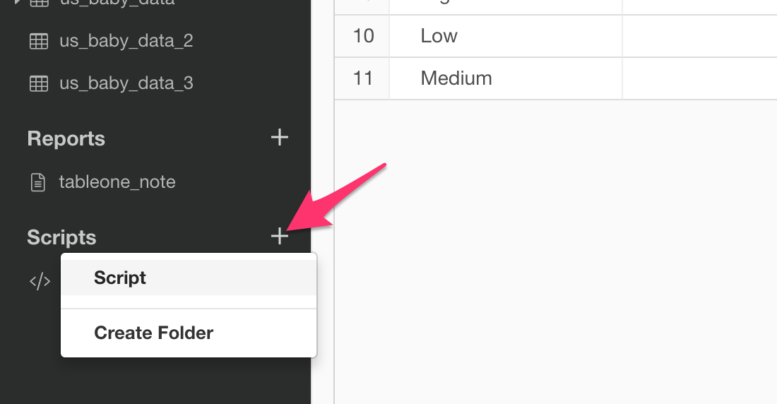
You can copy and paste the following script.
library(tableone)

run_tableone <- function(df, listVars, catVars, strata) {
  x <- CreateTableOne(vars = listVars, data = df, factorVars = catVars, strata=strata)
  as.data.frame(print(x)) %>%
    add_rownames("Name")

}
Once you save the script, then you can go to the data frame and call the ‘build_tableone’ function.
Select ‘Custom R Command’ from the Add button menu.
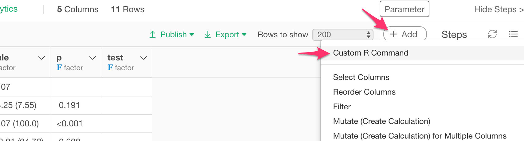
Here’s an example of calling ‘build_tableone’ function. It is setting which variables we are interested, which variables are categorical, and which variable to group the data.
run_tableone(c("Age", "Cholesterol",
"SystolicBP", "BMI", "Smoking", "Education"),
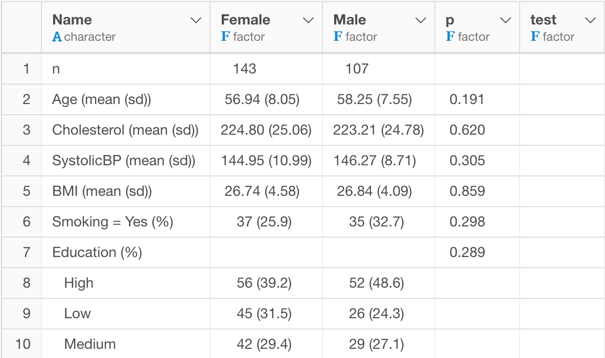
c("Smoking","Education"),c("Gender"))Once you run it, you’ll get the result like the below.
Data Wrangling with the output of tableone
You can clean up this data further by using various data wrangling techniques.
For example, we might want to separate the mean and the sd (standard deviation) into different columns. And you might want to make those Factor data type columns to Numeric columns.
Separate Columns
You can separate a column into multiple columns by selecting:
Separate -> Separate to Columns by -> Custom
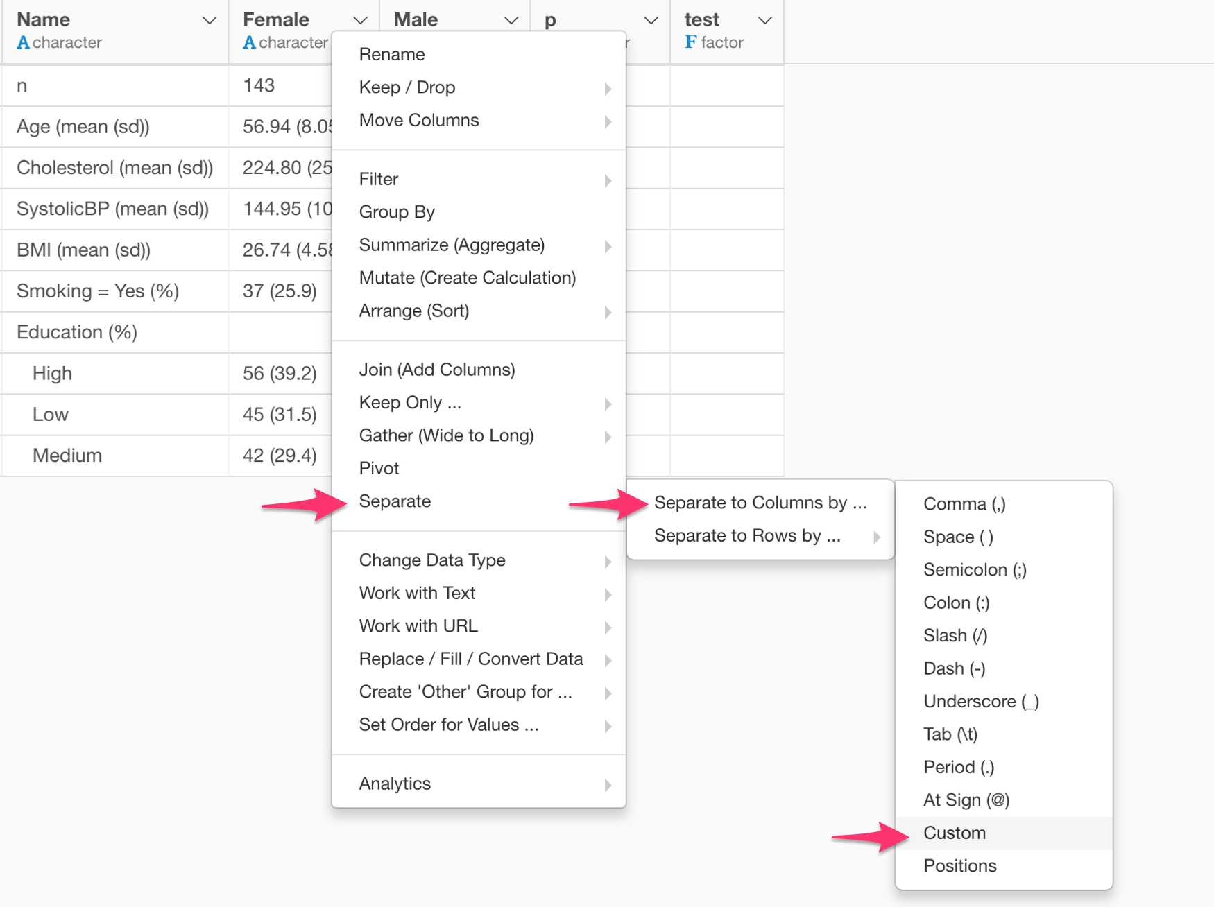
Type the following as the separator.
\(The backslash is an escape character for the bracket.
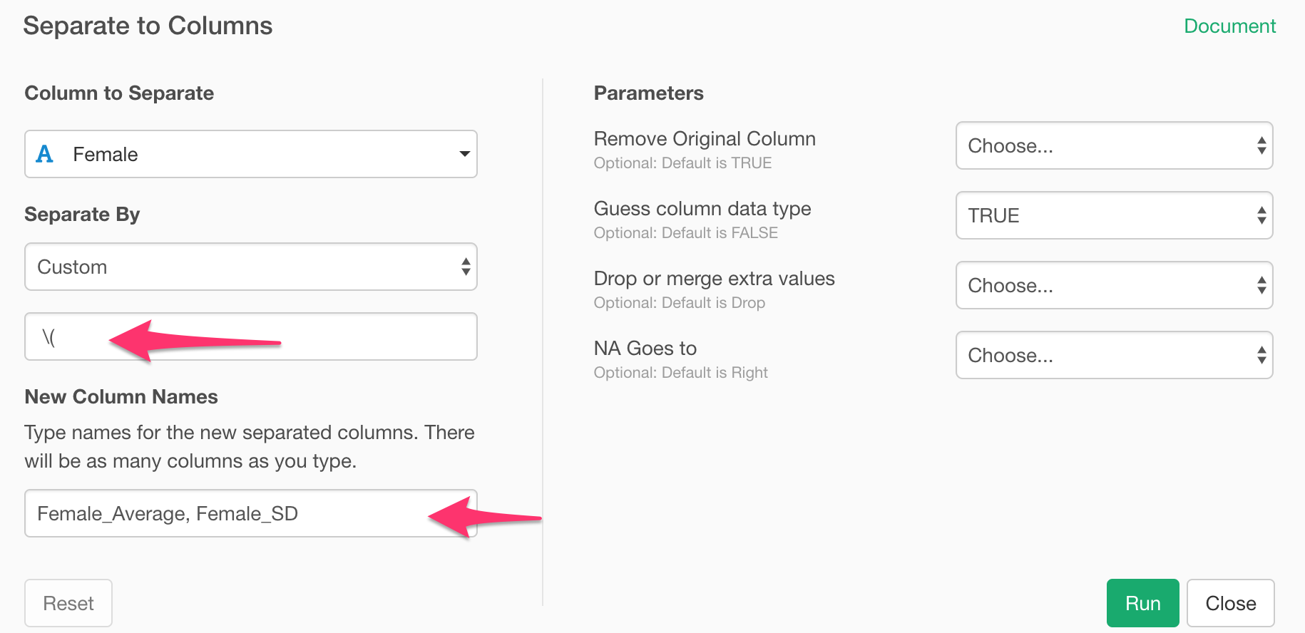
And you can type the newly created column names in the same dialog.
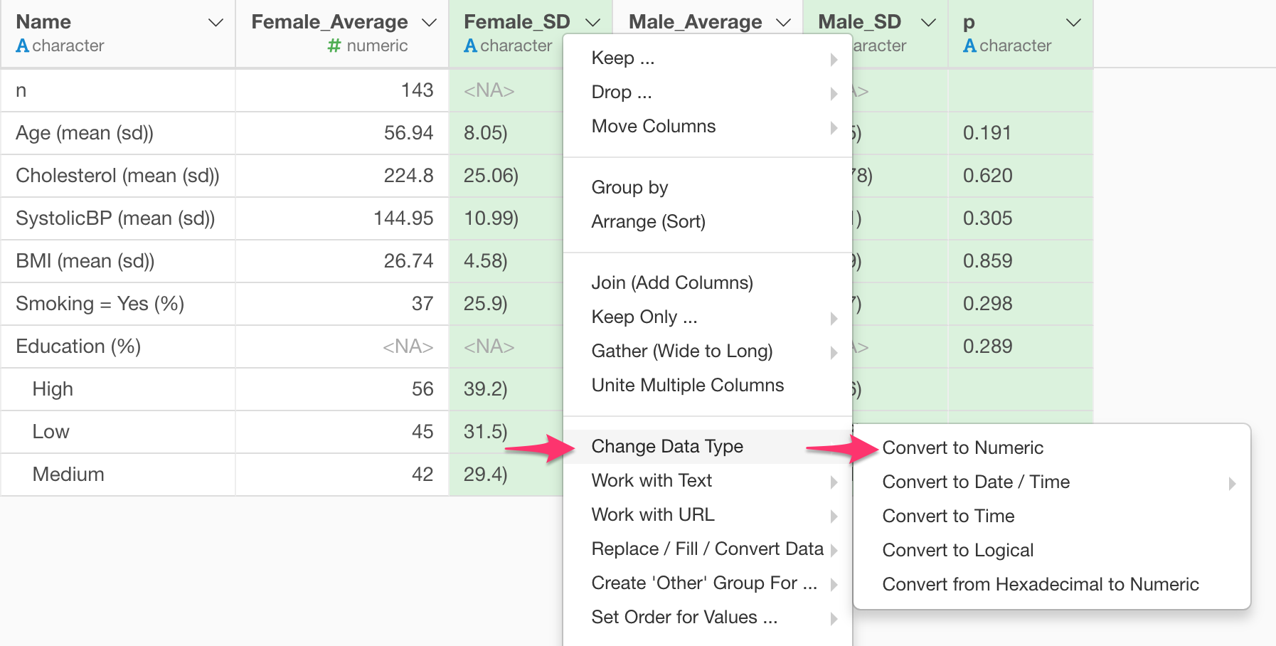
Convert from Factor to Numeric
You can convert some of the columns that are currently Factor or Character data type to Numeric. Select those columns by clicking the columns while pressing Command (Mac) or Control (Windows) key. Then, select:
Change Data Type -> Convert to Numeric
Here’s how it looks after a few steps of data wrangling.
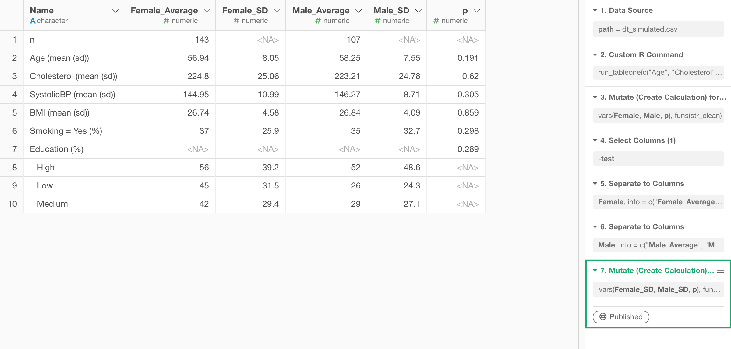
I’m sharing the data frame as EDF (Exploratory Data Format) so you can download it from this linkand import into Exploratory so that you can reproduce each data wrangling step. But, make sure you install ‘tableone’ R package and create an R script first by following the above steps before importing the EDF.