Introduction to Join Part 2 - Filter data based on another data frame

This is part 2 of ‘Introduction to Join’ series. You might want to take a look at part 1 first if you are not familiar with the basics of the Join feature.
- Introduction to Join Part 1 - Bring extra columns from the target - Link
Sometimes, you might want to filter your data based on the data from another data frame.
This is when you want to consider using ‘Filtering Join’ methods called Semi Join' or 'Anti Join' under Join family.
Note that these join types don’t bring the columns from the target data frame unlike other types such as Left Join. Instead, they use the target data frame's data only to filter the data, hence they are called 'Filtering Join.'
Let's take a look one by one.
1. Semi Join
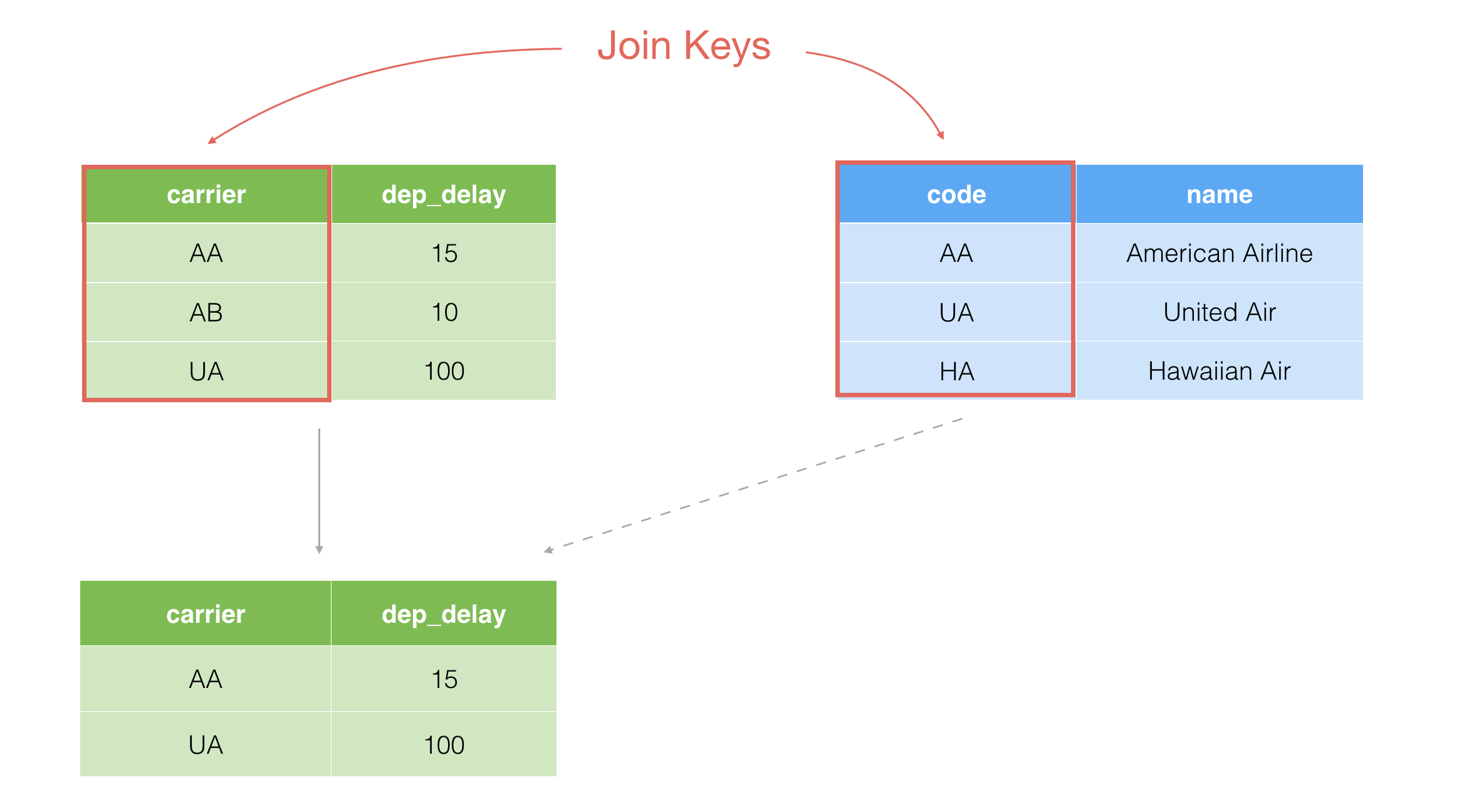
Semi Join is to keep only the rows in the current data frame that have the matching values in the target data frame.
In this example, there are AA and UA in the blue target data frame, therefore it ends up keeping only AA and UA rows in the main data frame after the join operation.
2. Anti Join
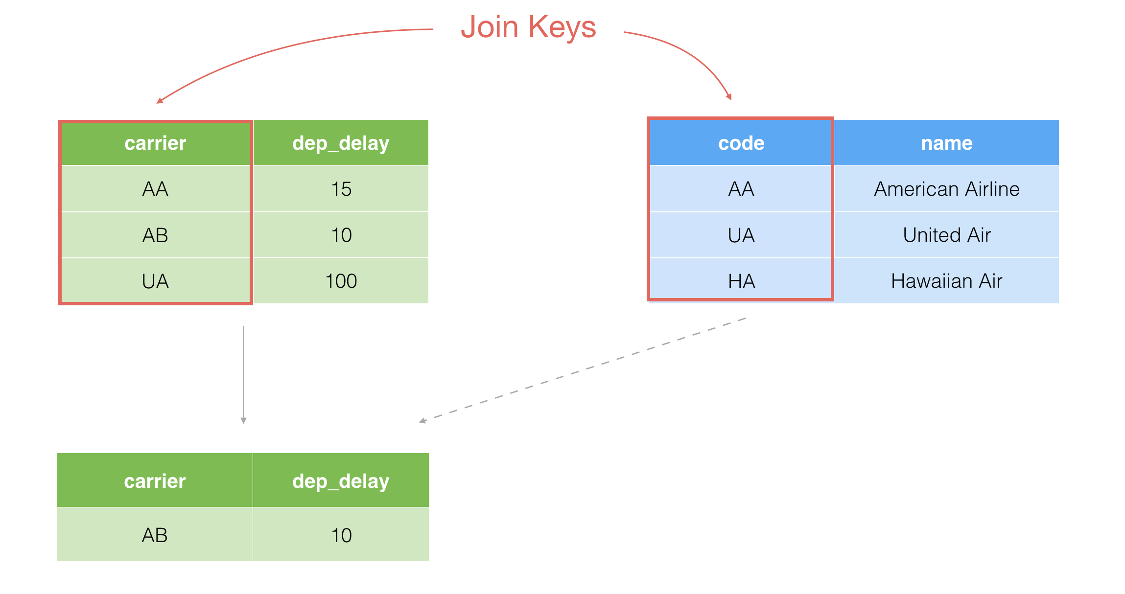
The opposite is Anti Join, which is to keep only the rows in the current data frame that don’t have matching values in the target.
In this example, carrier AB doesn't have its corresponding value in the blue target data frame, so it ends up keeping only AB in the result.
Now, let’s take a look at how these Join operations work using Exploratory.
Examples with Exploratory
Sample Data
If you are interested in trying out by your hands you can download the following data and follow the steps below.
- US Flight Delay Data - Link
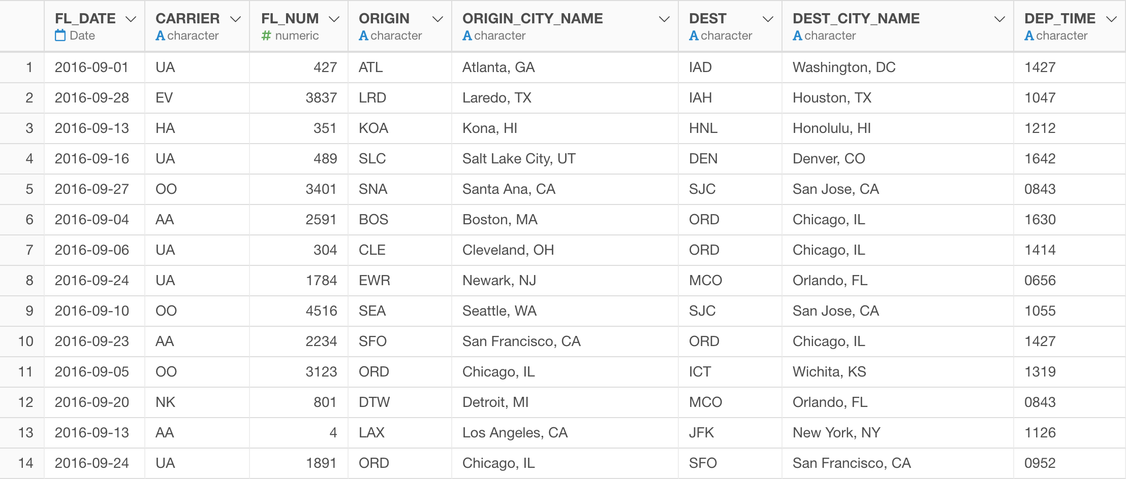
We have the US flight delay data like below.
Here is how the data looks like.
Keep the Data for Top 10 Cities
Let’s say, we want to see the flight delay data only for the top 10 most frequently cities.
1. Create Top 10 City List with Branch Data Frame
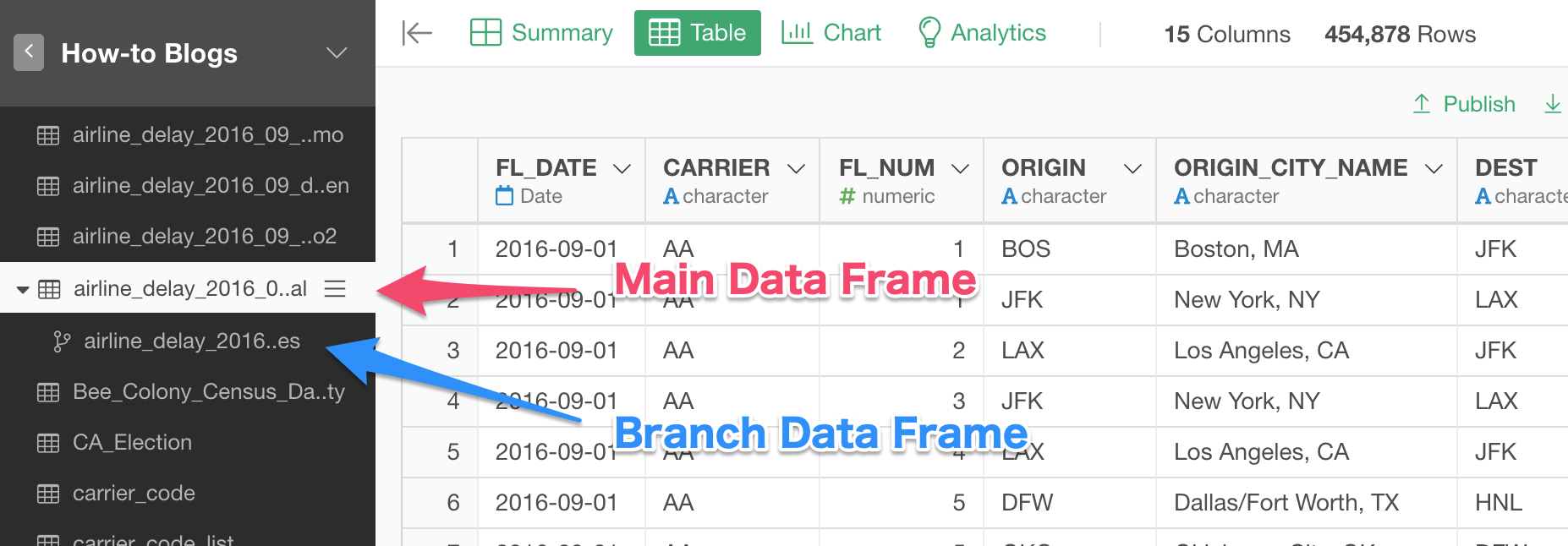
To do so, we can quickly create a branch data frame, which is basically a data frame branched off from the main data frame, and create the top 10 frequent city list.
- Introduction to Branch Data Frame - Link
Click 'Create Branch Data Frame' button in the step that you want the new branch data frame to start from.
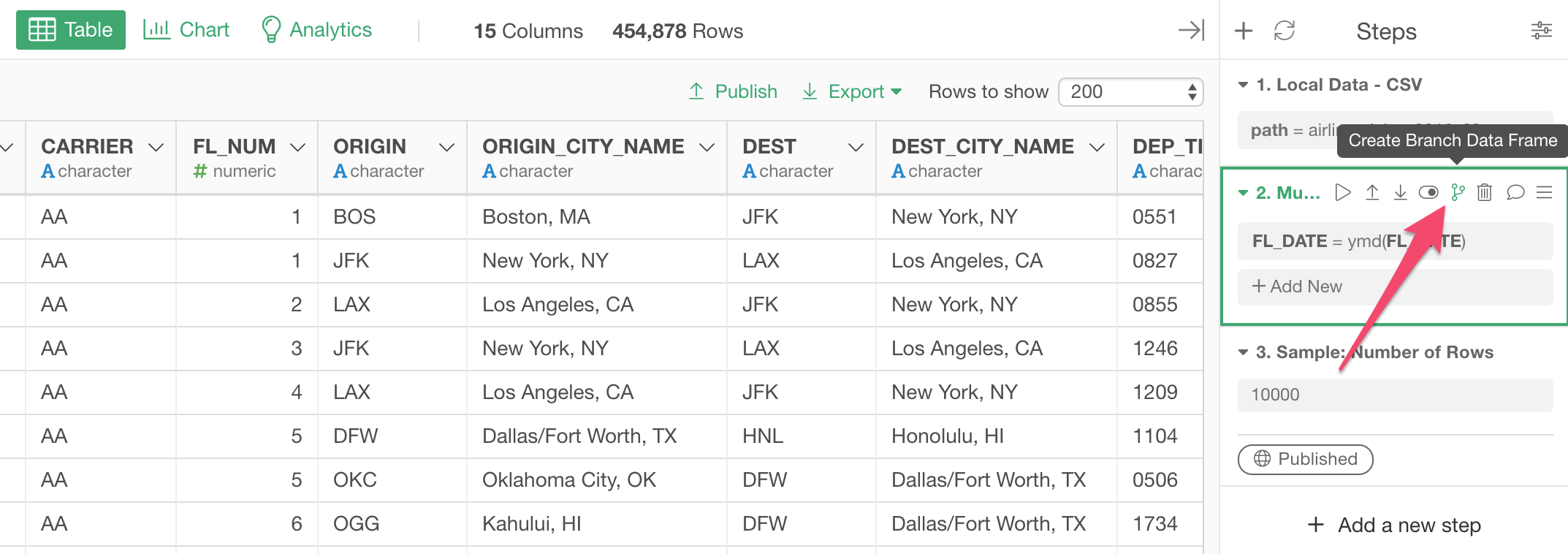
And, in the newly created ‘branch’ data frame, we want to do two things. The 1st step is to calculate the number of flights for each city with Summarize command. Then the 2nd step is to keep the top 10 cities with Top_N command.
2. Summarize Data to Count the Number of Flights
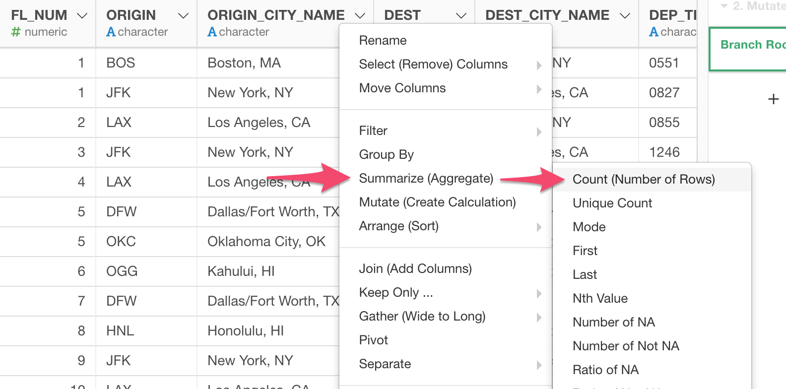
Select 'Summarize' and 'Count' from the column header menu.
Select 'ORIGIN_CITY_NAME' as the grouping column.
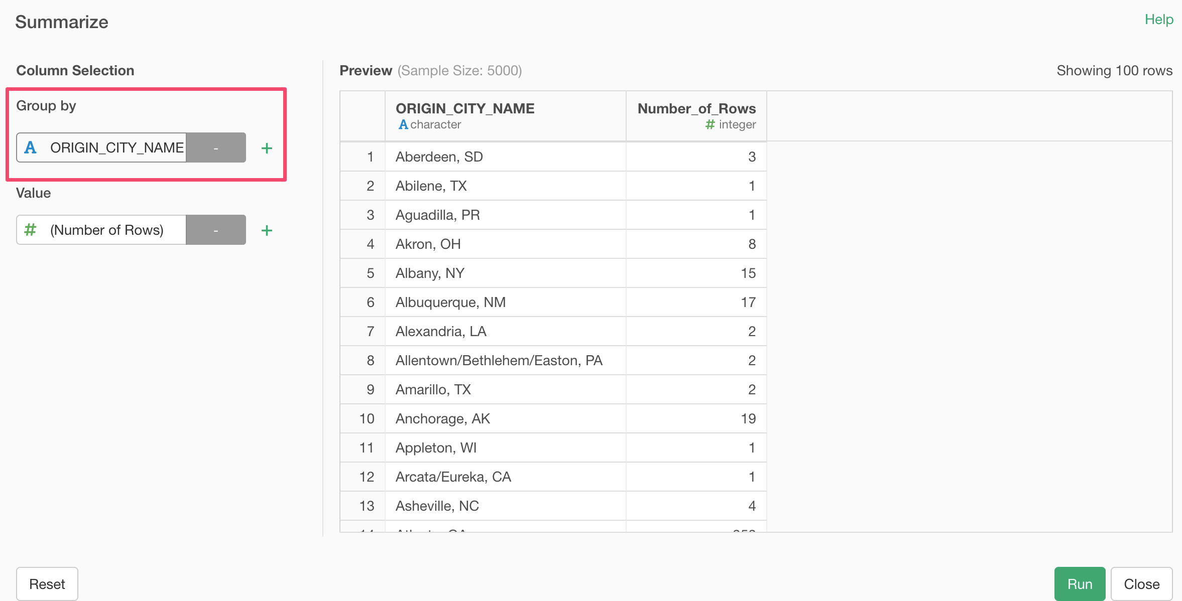
This will calculate the number of flights for each city (origin city, the city that flights departed from.)
3. Keep Only Top 10 Cities
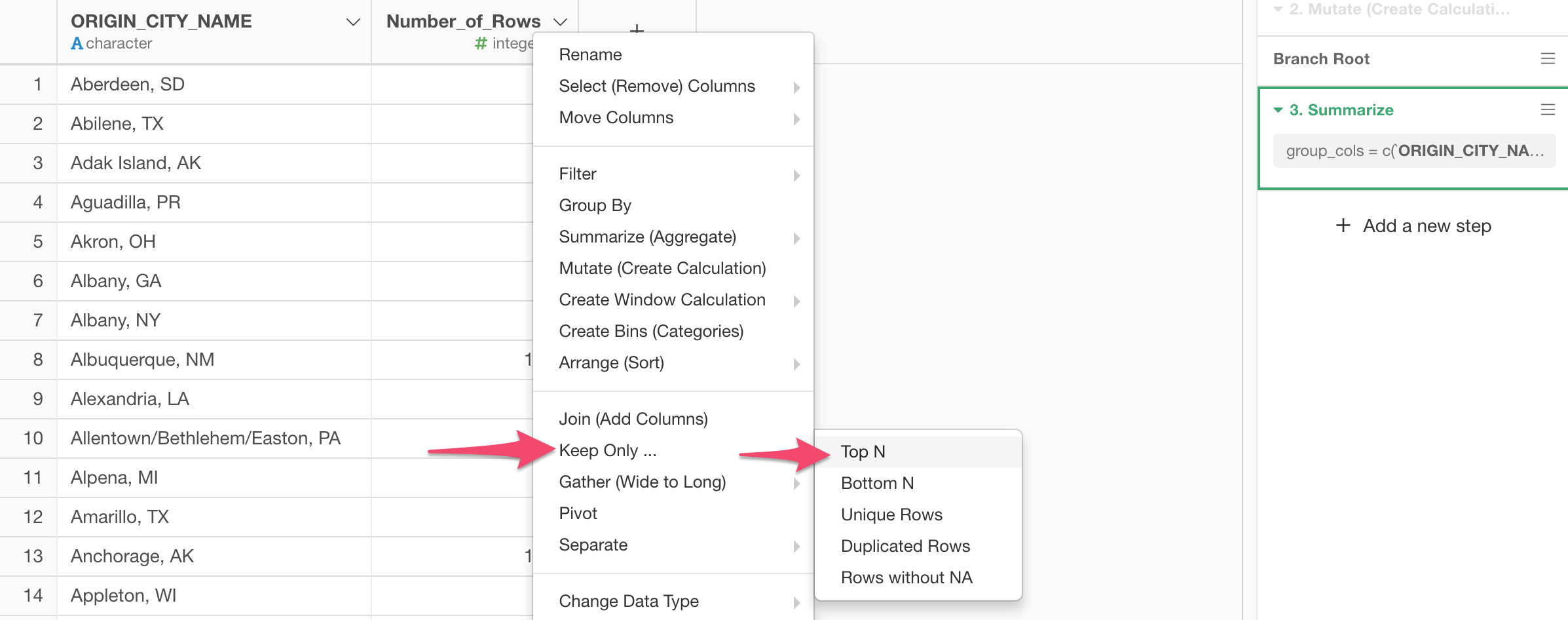
Select 'Keep Only' and 'Top N' from the column header menu.
Make sure that '10' is entered to make it as Top 10.
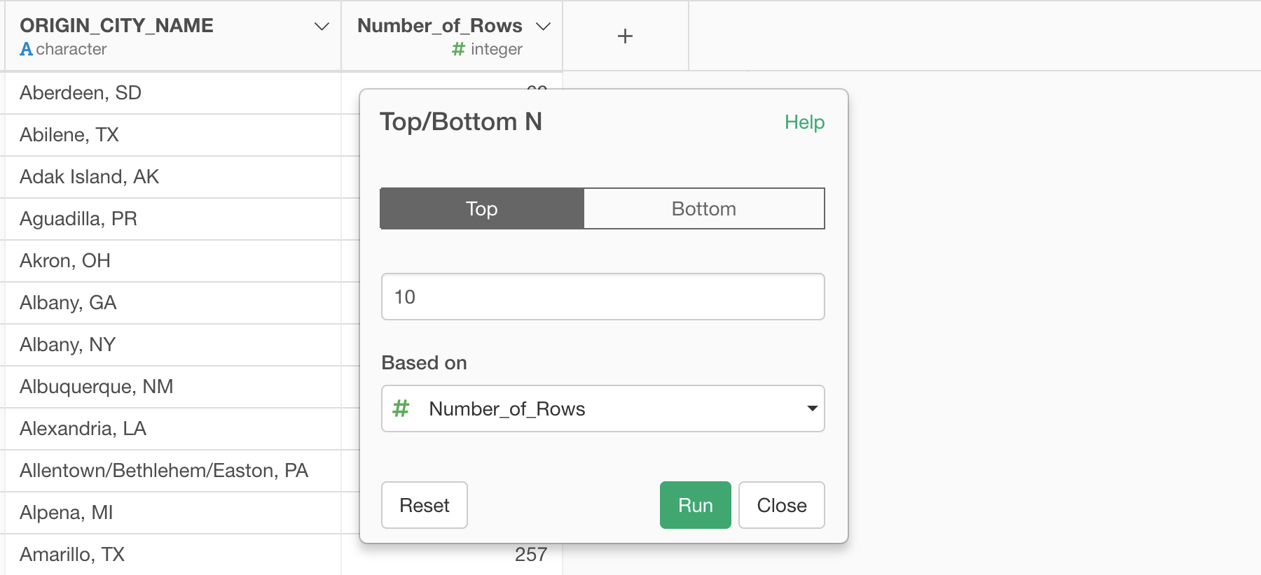
Once you run it you will get only the top 10 most frequent cities.
4. Use Semi Join to Filter Data Using Top 10 City List
Now, go back to the main data frame.
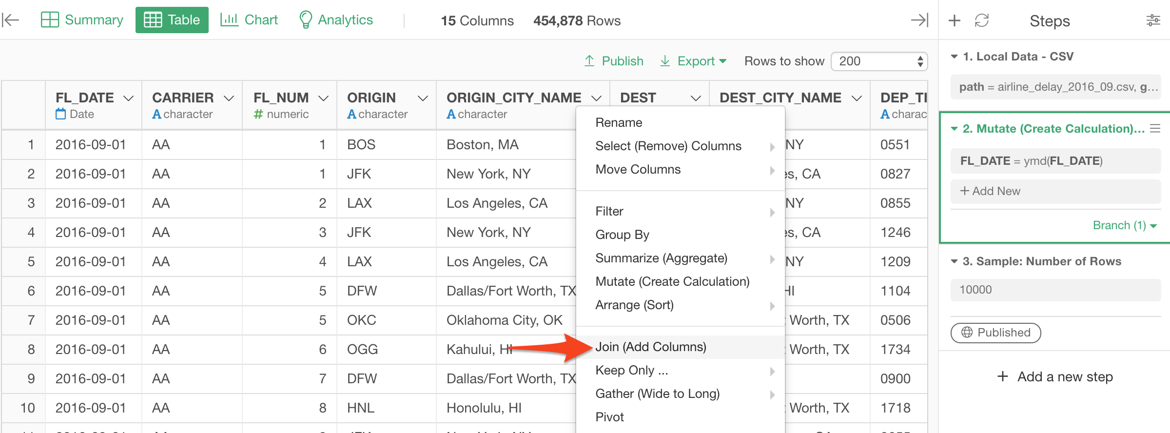
Then, select 'Join' from the column header menu.
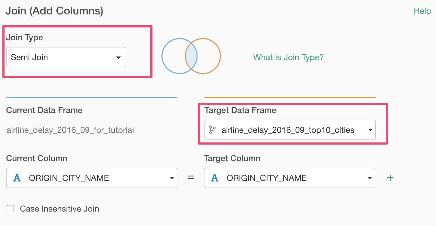
Select 'Semi Join' as the Join Type and select the branch data frame we have just created.
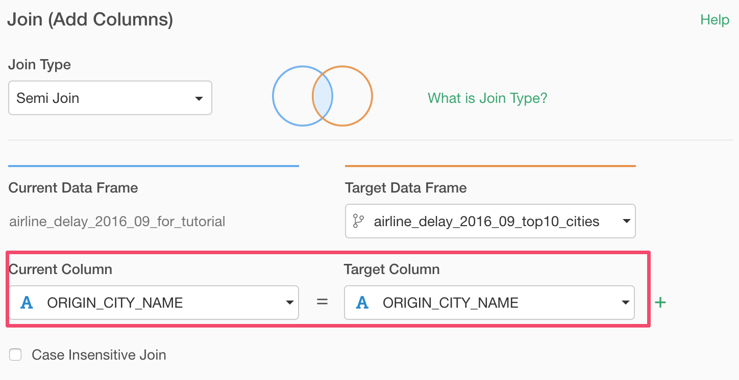
Make sure ‘ORIGIN_CITY_NAME’ column is selected for both Current and Target column selections, to match the two data frames' data.
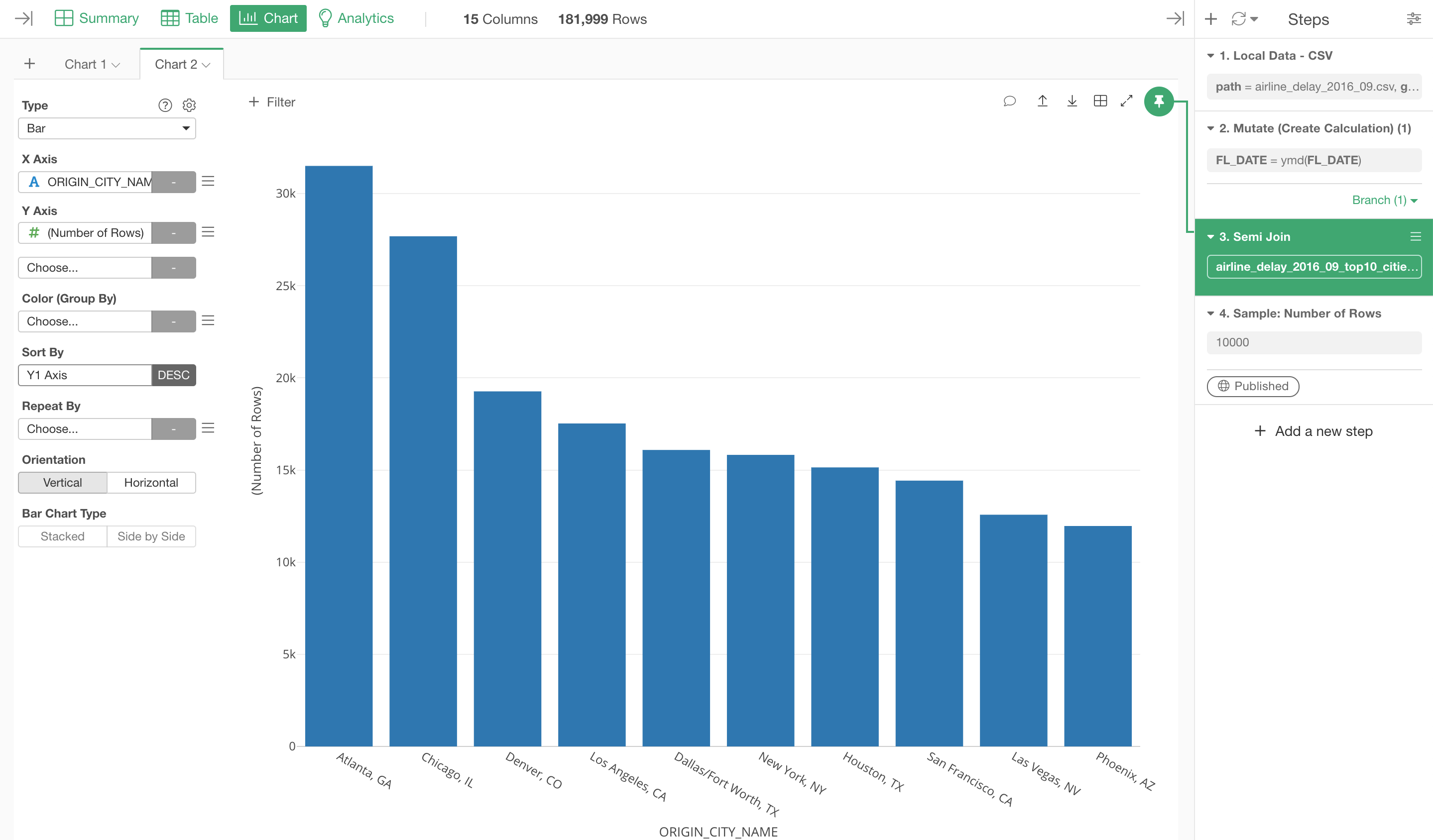
We can quickly visualize the top 10 cities by using one of the charts.
If you move the Pin button to the previous step before the 'Join' step by drag-and-dropping the button, then the same bar chart will show all the cities.
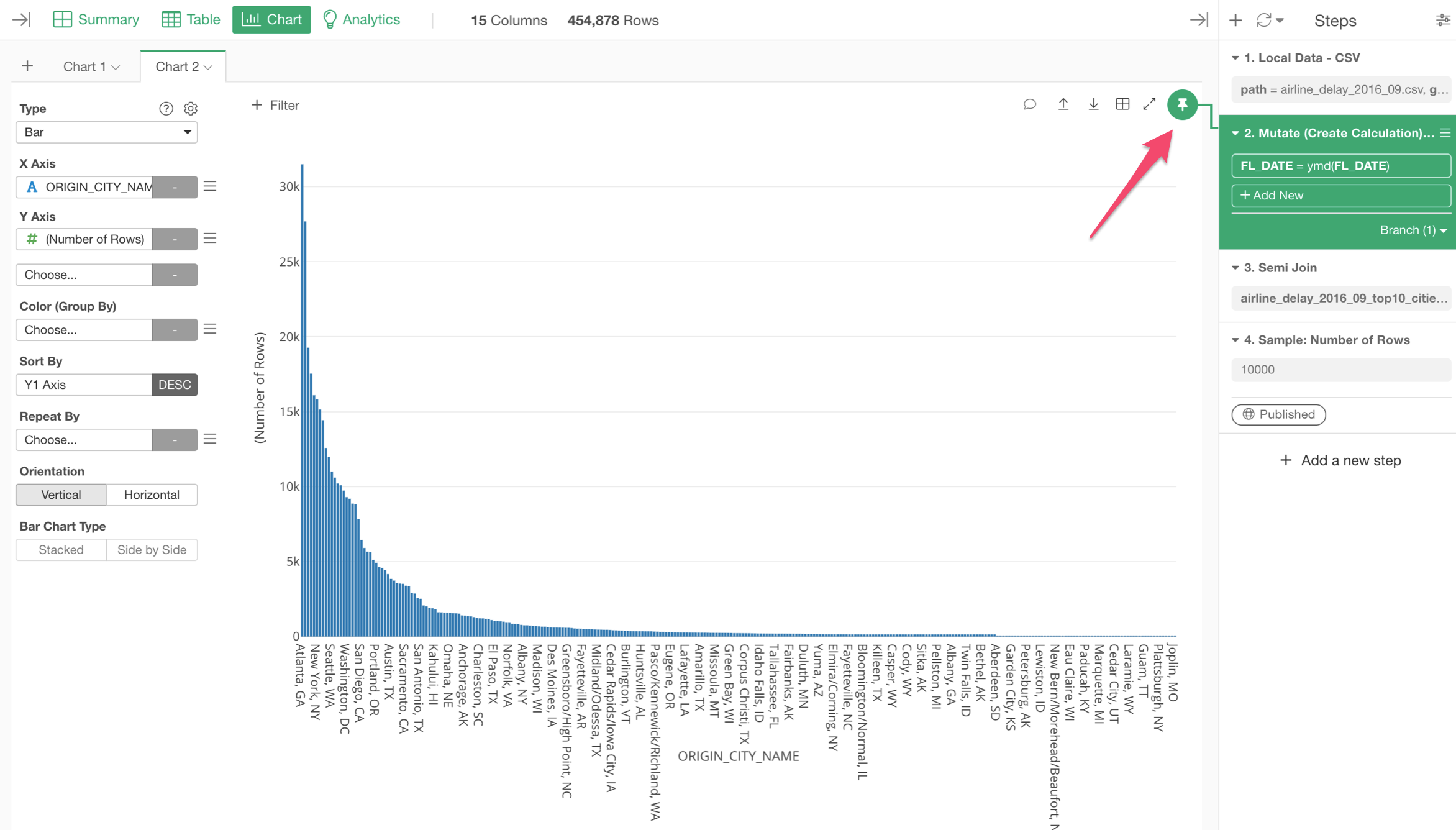
- Introduction to 'Pin' feature in Chart - Link
Keep the Data for Non-Top10 Cities
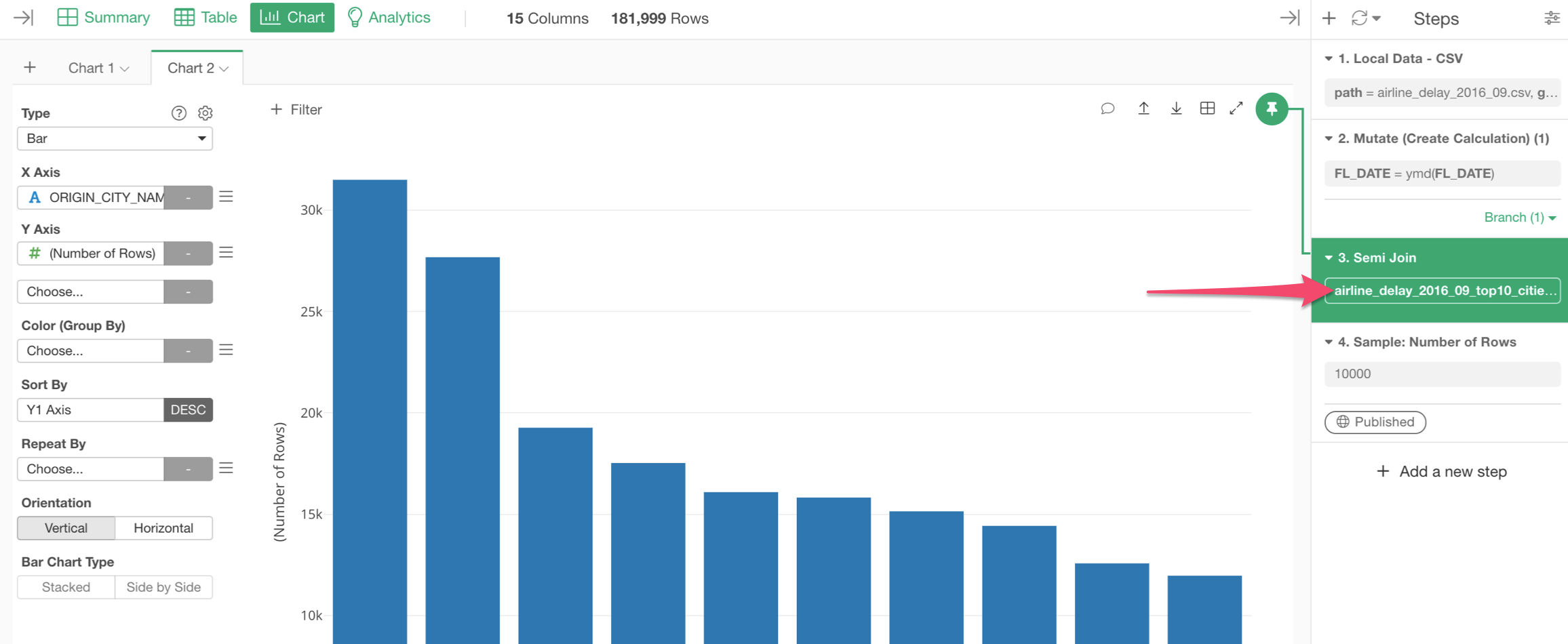
Bring the Pin button back to the Join step to show only the top 10 cities.

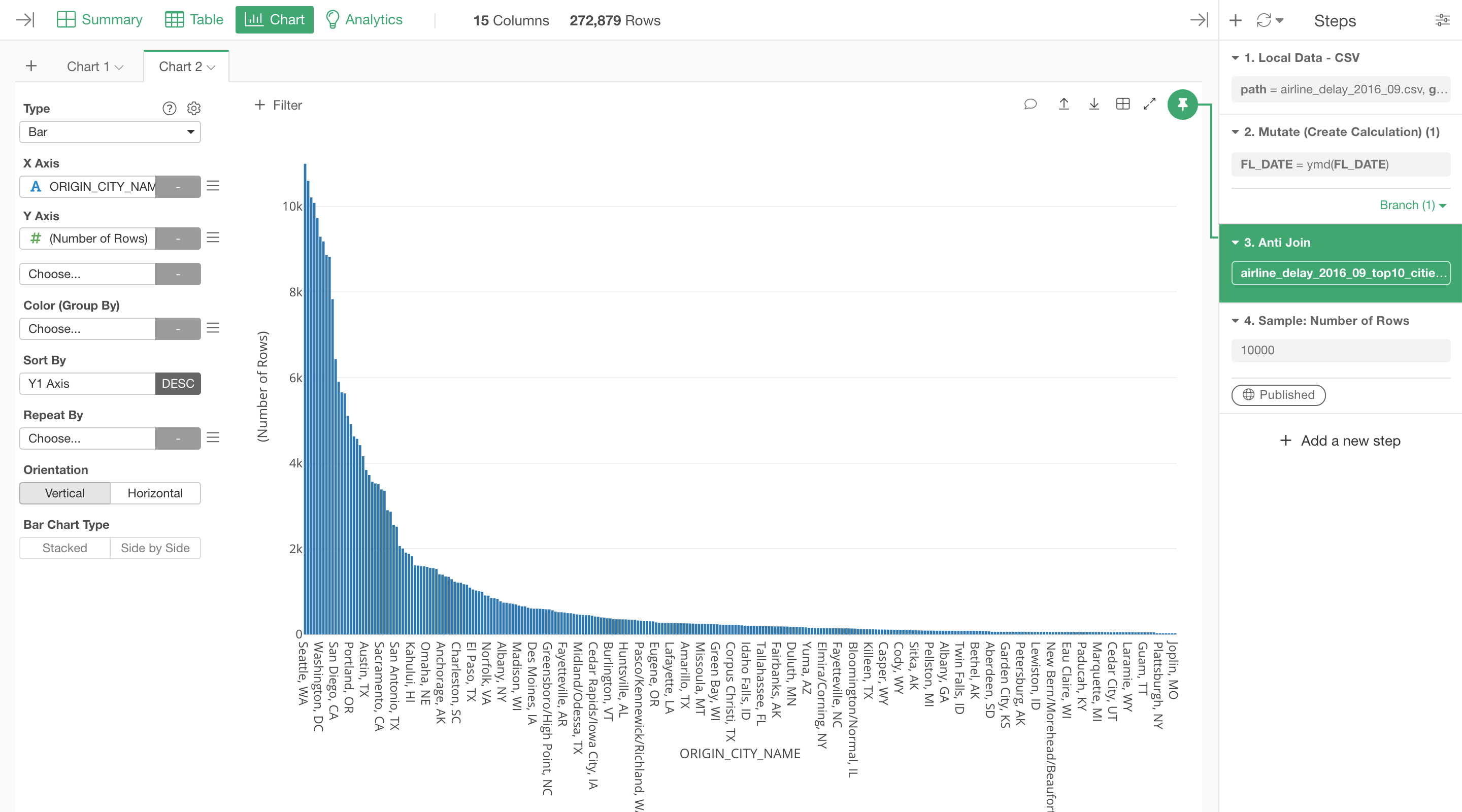
Now, let's say, for some reasons, we want to show the data only for the NON top 10 cities.
You can click on the token button inside the 'Join' step to open the 'Join' dialog.
And select 'Anti Join' as the Join Type.
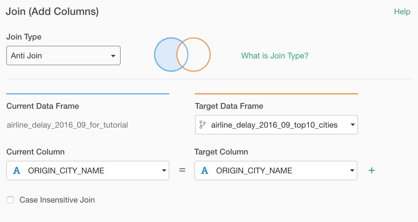
Once you run it, you will see only the Non top 10 cities data in the chart.
Make sure to check out the Part 1 of this Join series, if you haven't yet!
- Introduction to Join Part 1 - Bring extra columns from the target - Link