Why is Multicollinearity a Problem When Building Statistical Learning Models?

When you are building statistical learning models you don’t want to have variables that are extremely highly correlated to one another because that makes the coefficients of the variables unstable.

And when the coefficients are unstable, we can’t rely on the coefficient information, which is the most important piece of information you can get out of the models.

Let’s say we have Employee Salary data and want to build a linear regression model to predict Salary based on Job Level and Working Years.

Here is a formula of the linear regression model.

And, by building the model we can find out the above parameters a, b, and c.

Let’s say we’ve got the following parameters.

This means that one level increase in the Job Level will have a $500 increase in the Salary when the Working Years stay the same. Similarly, a year increase in the Working Years will have a $100 increase in the Salary if the Job Level stays the same.

Now, as it turned out that the Job Level is actually decided based on the Working Years in this company and there is a formula they use to decide the Job Level like the below.

This means that once we know the Working Years of an employee we know what is her Job Level.

For example, if this person’s working years is 10, then her job level can be calculated as 3 by using the above formula.

Now, if we had such a relationship between the Job Level and the Working years, the following three linear regression formulas would end up producing exactly the same salary value.

They all produce 4,000.

And this is a problem because the coefficients of the Job Level and the Working Years are not reliable.

One year increase in working years will make your salary $100 more? or $200 more? Or maybe $0!

Now that we know that multicollinearity is a problem to watch out for, how can we detect it methodically?

Can we detect such relationships in predictor variables?

Detecting such a relationship in the predictor variables is actually pretty simple.

Do you remember that when we have the multicollinearity problem we should be able to define the relationship between the predictor variables like the following formula?

When you look at this formula, you’ll notice that this is a linear regression formula to predict Job Level based on Working Years.

So far, we are assuming this is a perfect formula.

But it doesn’t have to be this perfect.

Linear Regression models always have the residuals, which is the difference between the estimated values by the model and the actual values.

Let’s call this an ‘error’.

Then, we’ll have a linear regression formula like the below.

So, if this formula’s error is very small, it means that the Job Level and the Working Years are in a highly correlated relationship. And that’s the relationship of ‘if you know the answer of one variable and you’ll know the answer for the other.’.

And one way to measure how small the error of this model is to calculate the R-Squared.

The R-Squared is a measure of how good a given model can explain the variance of the target variable.

It ranges between 0 and 1. As it gets closer to 1 the correlation between the target and predictor variables is considered to be higher. As it gets closer to 0 there is not much correlation between the two variables.

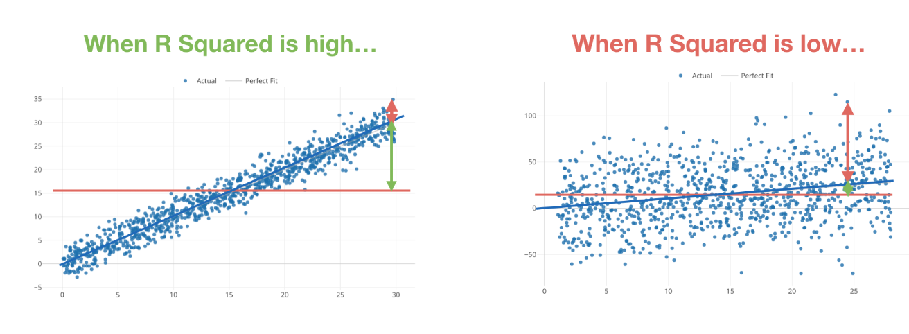
So, we can build a model with the Job Level as the target variable and the Working Years as the predictor variable and measure the R-Squared to see how much they are correlated.

If it’s closer to 1, then we can say that Job Level and Working Years are highly correlated. And this means that having both of them as predictor variables could cause the multicollinearity problem.

On the other hand, if the R-Squared is low, then these two variables are not well correlated. Hence, we don’t need to worry about the multicollinearity problem for having them as predictor variables.

And this is the basic logic of how we can detect the multicollinearity problem at a high level. But let’s see a bit more details.

Detecting Multicollinearity by Measuring R-Squared

In order to detect the multicollinearity problem in our model, we can simply create a model for each predictor variable to predict the variable based on the other predictor variables.

Let’s say we want to build a linear regression model to predict Salary based on Job Level, Working Years, and Age like the following.

And we want to find out if we have the multicollinearity problem among the predictor variables of Job Level, Working Years, and Age.

Then, we can build a model for each predictor variable to predict the values based on other predictor variables like below.

And we can measure the R-Squared for each model. If the R-Squared for a particular variable is closer to 1 it indicates the variable can be explained by other predictor variables and having the variable as one of the predictor variables can cause the multicollinearity problem.

Now, let’s assume we have the following R-Squared calculated for each model.

The first one’s R-Squared is 0.99, and it tells us that the Job Level can be explained almost perfectly by the Working Years and Age. This indicates that having the Job Level most likely to cause the multicollinearity problem.

By the way, we don’t know if the Job Level is correlated with the Working Years or with the Age from this model alone. But if the Job Level and the Working Years are highly correlated then the R-Squared for this model should be high regardless of whether the Job Level is correlated with the Age or not.

Now the second one’s R-Squared is 0.90, and it tells us that the Working Years can be explained by the Job Level and the Age pretty well. This indicates that the Working Years might cause the problem, but the evidence is not as strong as the first one.

The last one’s R-Squared is 0.70, and it tells us that the variance of the Age can be explained by the Job Level and Working Years, but only 70% of it. This indicates that the Age is not going to cause the problem.

So, by building the models for every single predictor variable and measuring the R-Squared for each we can detect the multicollinearity problem.

As we have seen so far, the R-Squared can be our guide for detecting the multicollinearity problem. But there is another measure called VIF (Variance Inflation Factor) that is often used as a measure of detecting the multicollinearity problem.

What is VIF?

VIF (Variance Inflation Factor)

VIF is nothing but the inflated version of the R-Squared.

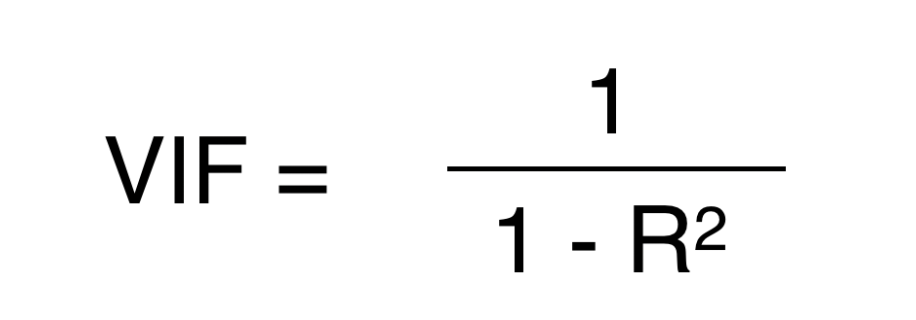
Honestly, I’m not completely convinced on why we really need to inflate the R-Squared, but I’m guessing that it makes it easier to see the differences as the R-Squared gets closer to 1. (please leave your comments if you know a better explanation.)

Anyway, we can calculate the VIF for the above models as below.

As you can see when the R-Squared getting closer to 1 the VIF becomes huge.

The general guideline is that when the VIF goes beyond 10, which means that the R-Squared is 0.90, there is a risk of having the multicollinearity problem.

What should we do when we got Multicollinearity?

Now, what are we going to do when we have the multicollinearity in our model? Just remove one of the variables with high VIF, rebuild the model, and see if it still has such a problem.

How are we going to decide which variables to remove?

That really depends on what you’re interested in.

In the above example, you want to remove either the Job Level or the Working Years. If you are interested in understanding the relationship between the Job Level and the Salary then keep the Job Level but remove the Working Years.

Now, let’s take a look at an example use case. I’m going to use Exploratory (UI tool to do Data Science) to demonstrate.

Working to Address Multicollinearity in Exploratory

Here is a quick example.

I had an employee salary data and wanted to build a linear regression model to explain how the salary changes based on a given set of employee attributes such as Age, Gender, Working Years, etc.

So I built one, and here is the Coefficient tab showing the coefficients of all the predictor variables.

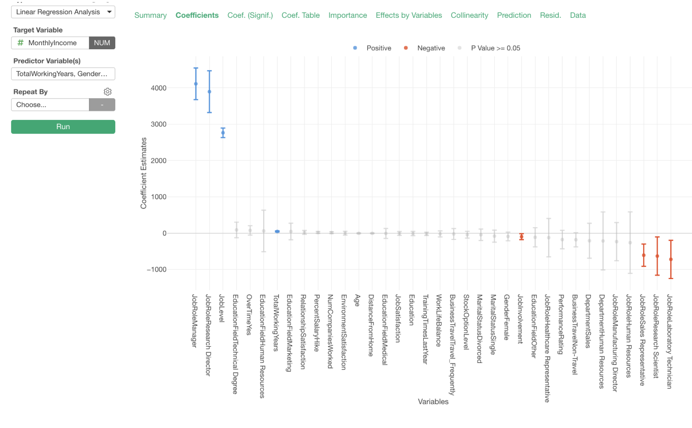
Now I want to make sure this model doesn’t have the ‘multi-colinearity’ problem. If it has then I can’t rely on these coefficients.

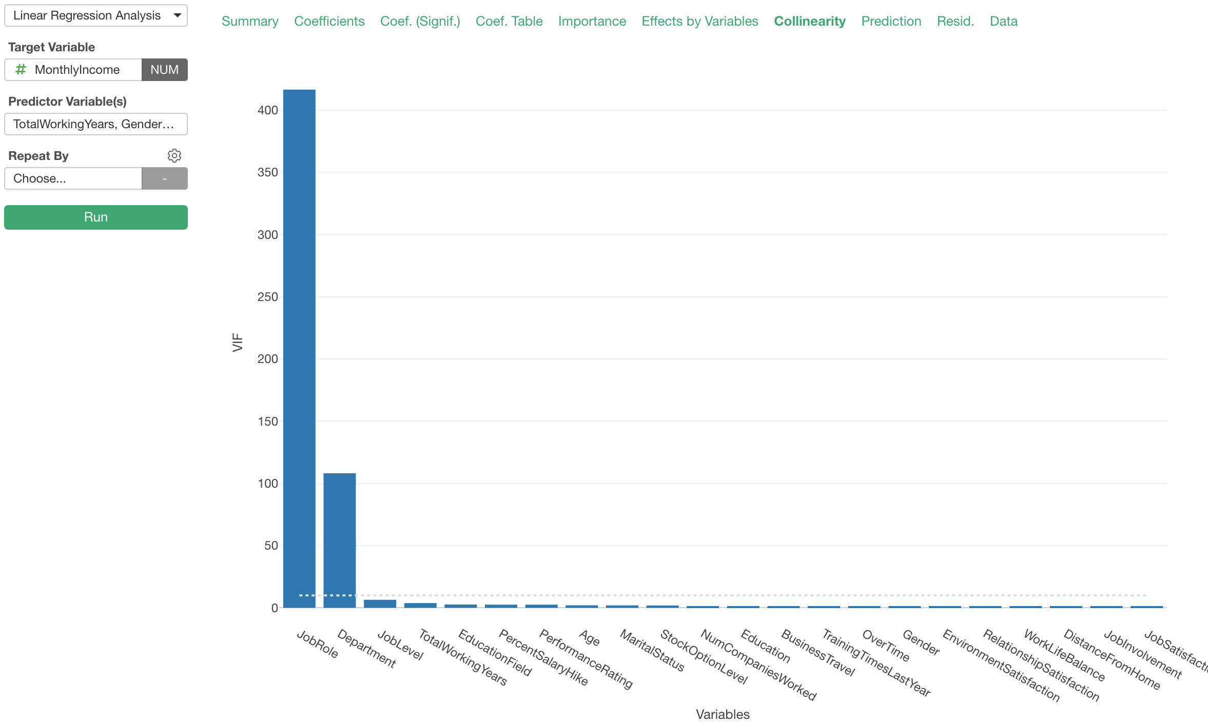
We can go to the ‘Colinearity’ tab to check if there are any variables that might be at risk of causing the ‘multicollinearity’ problem.

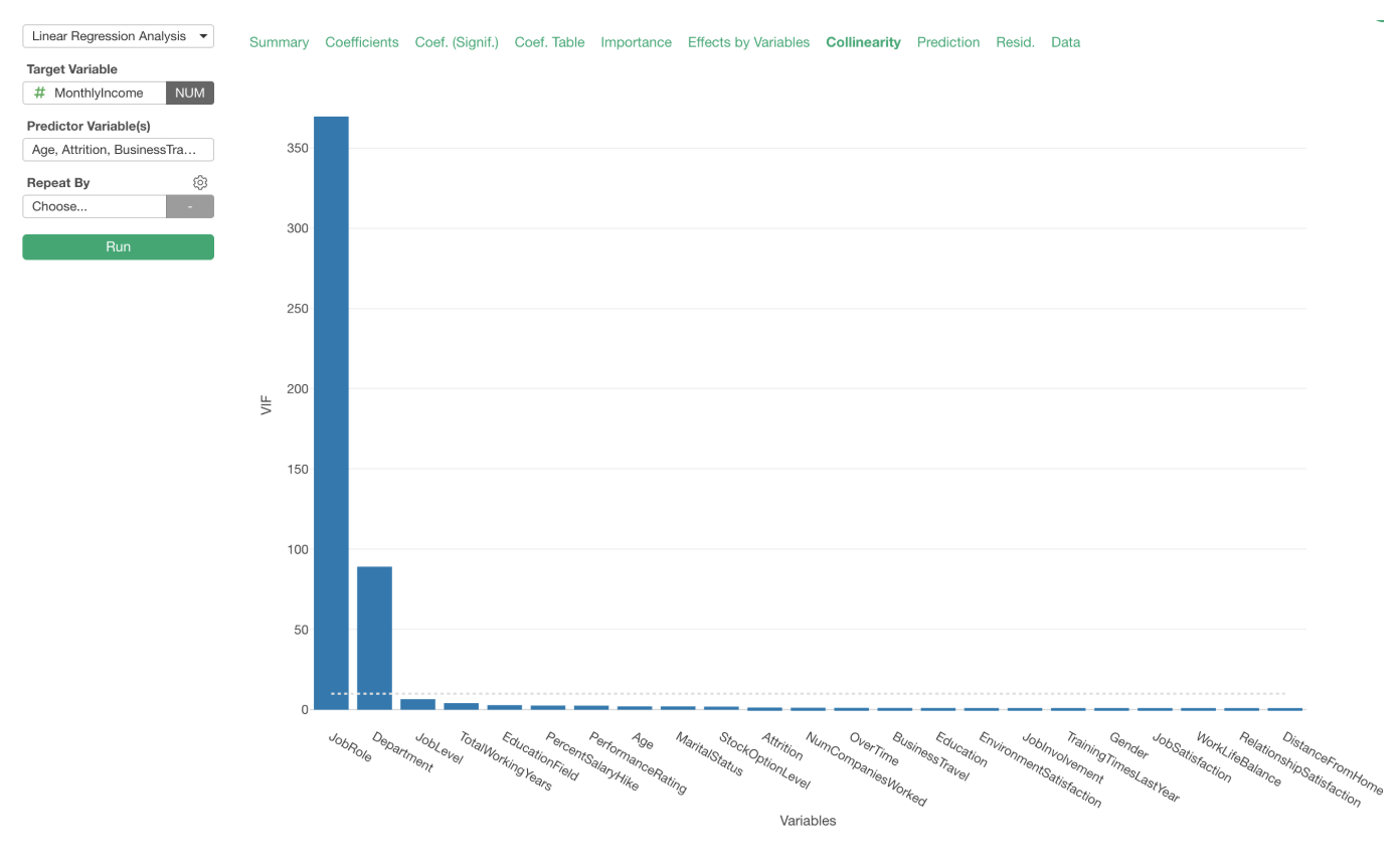
When you run a linear regression model in Exploratory it automatically does the logic I explained above, which is to create a linear regression model for every single variable and measure the R-Squared and VIF, behind the scene so you don’t have to do it manually. 💪

Now, the Collinearity bar chart above is showing the ‘VIF (Variance Inflation Factor) for each predictor variable.

We can see that ‘Job Role’ and ‘Department’ variables have very high VIF values, which indicates that they are causing the multicollinearity problem.

By looking at the relationship between the Job Role and the Department by using the Bar chart, we can see that they are super associated with one another.

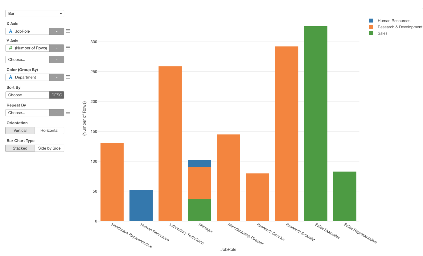
Except for the case of ‘Manager’, you can perfectly know which department a given employee belongs to once we know their ‘Job Role’.

This is why the VIF for these two variables are high. It’s always a good practice to visualize such a relationship so that you can understand it intuitively.

Anyway, as long as we have these two variables as part of the predictor variables together the coefficients are not stable, hence we can’t rely on them.

So, which one to remove? Job Role or Department?

That depends on what we want to know.

For this example, let’s say we are interested in the Job Role more than the Department so we’ll remove the Department and re-build the model.

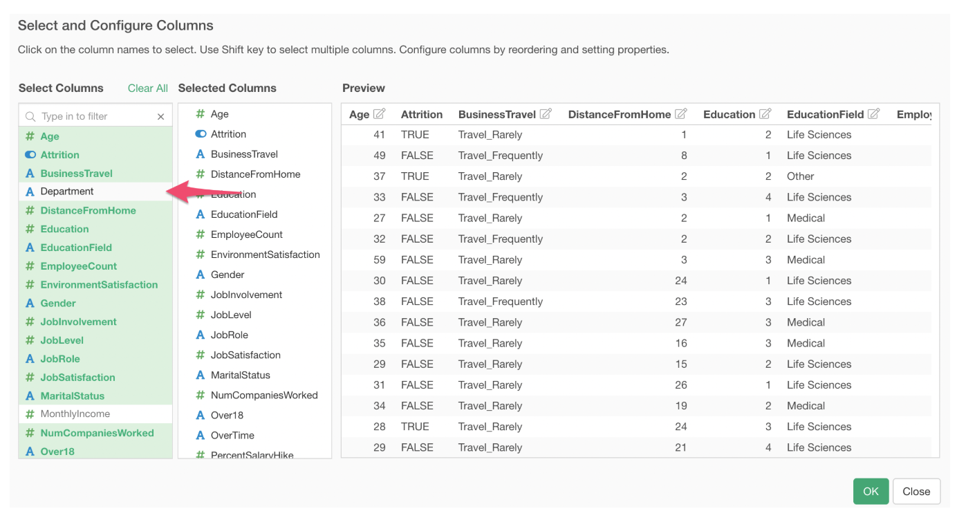
Now that we don’t have the variables with extremely high VIF values.

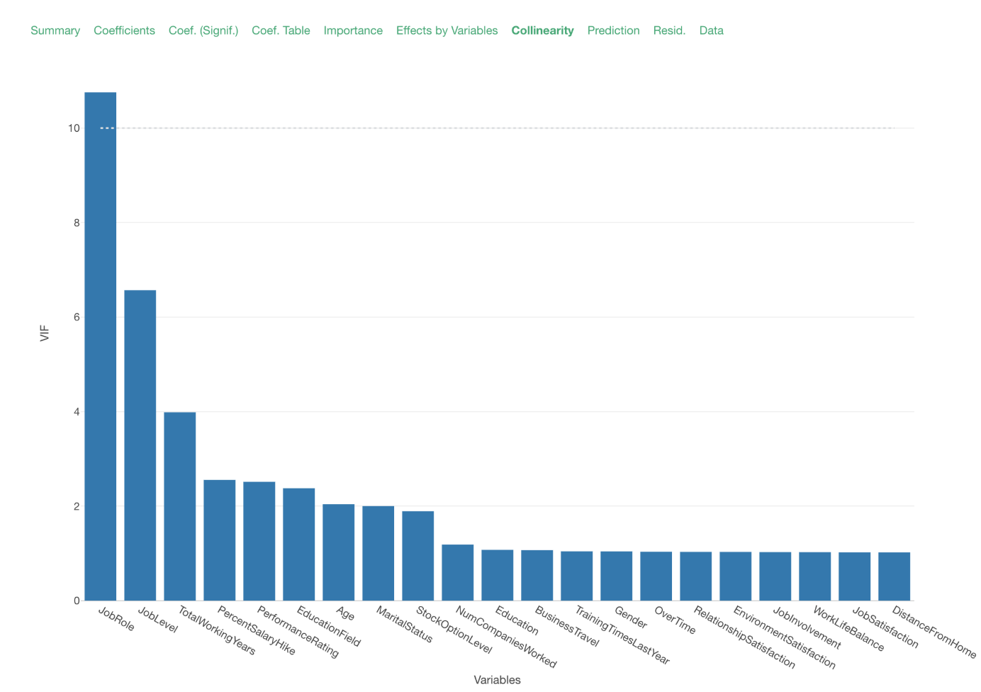
The ‘Job Role’ VIF is 10.76, which is relatively high. This indicates that about 90% of the variance of ‘Job Role’ can be explained by the other predictor variables. We can remove this variable, but then we won’t be able to answer the question of how ‘Job Role’ is associated with the monthly income.

Given that the VIF is not extremely high, I’m going to keep it and continue on the analysis of how the monthly income is correlated with the other employee attributes.

Now, one last thing.

So far, we have looked at how to detect and address the multicollinearity problem methodically by using a given data.

But also it is always a good practice to ask about such a relationship that is detected as ‘multicollinearity’ to the ones who know the data and the business rules behind it. They will tell you if there are indeed such business rules behind the relationship if any.