Reverse Geocoding Part 1 — Using Boundary Data with GeoJSON
Suppose if you have a set of longitude and latitude pairs, and you want to know the location names such as States, Prefectures, etc. This is called ‘reverse geocoding’, as opposed to ‘geocoding’ which maps geocodes (longitude and latitude) based on the addresses. And, there are a couple of ways to do this. Each option has pros and cons, but today I’m going to show you how to do it by using GeoJSON files.
GeoJSON is a format for encoding a variety of geographic data structures. It is often used to draw a boundary of countries, regions, states, cities, and others. In Exploratory, we use those GeoJSON for data visualization.
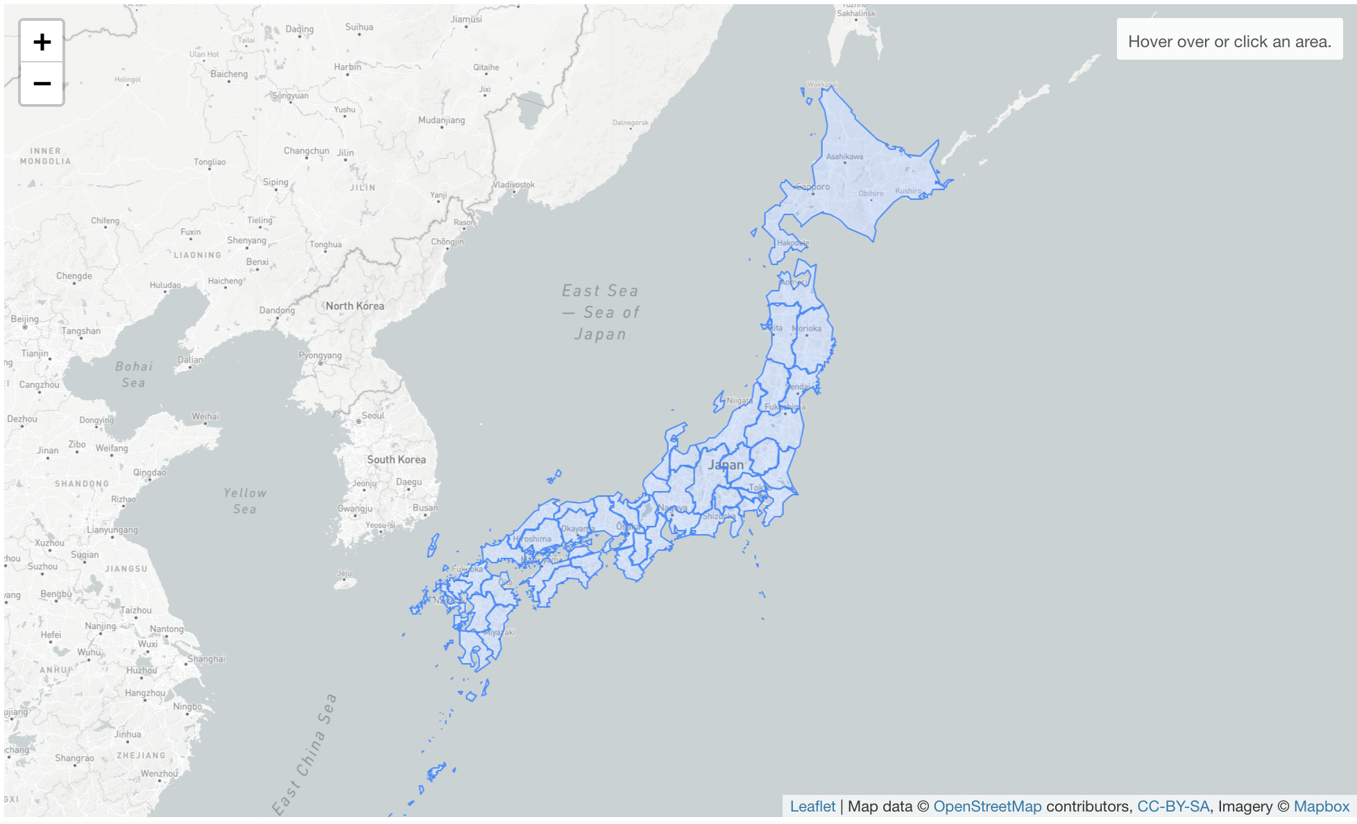
GeoJSON consists of a set of groups, Japan’s prefectures above. Each group has a set of coordinate info to draw a polygon shape, like the shape of Tokyo prefecture. You can look at the Wikipedia page about the GeoJSON for more detail if you are interested. Anyway, you can check which boundary a given geocode point (longitude / latitude) is located inside to map it to a corresponding name of the boundary such as Prefecture.
And thanks to R community, yes you can do this with the sf package. I'm going to explain how to do it with Exploratory.
Install sf package
The sf package doesn't come with the Exploratory, so you need to install it first.
First, select "Manage R Packages" menu from the project menu. 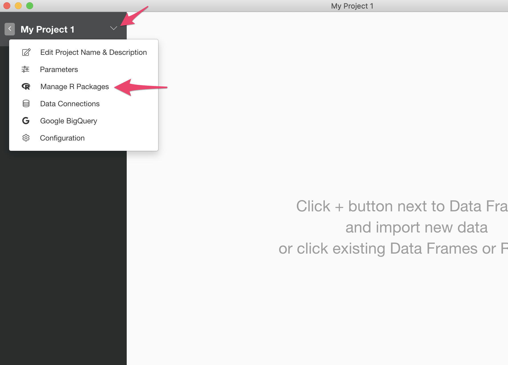
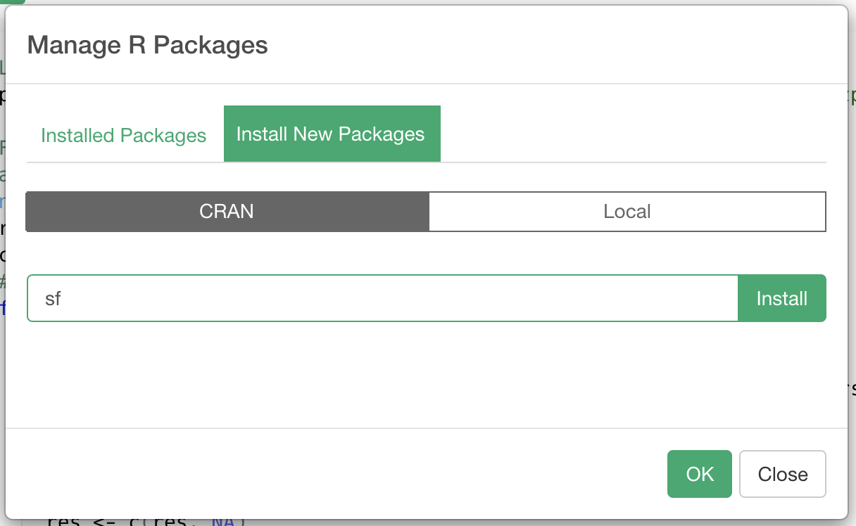
It opens up the R Package management dialog. Click "Install" tab, and type in "sf" in the text box, and click "Install" button.
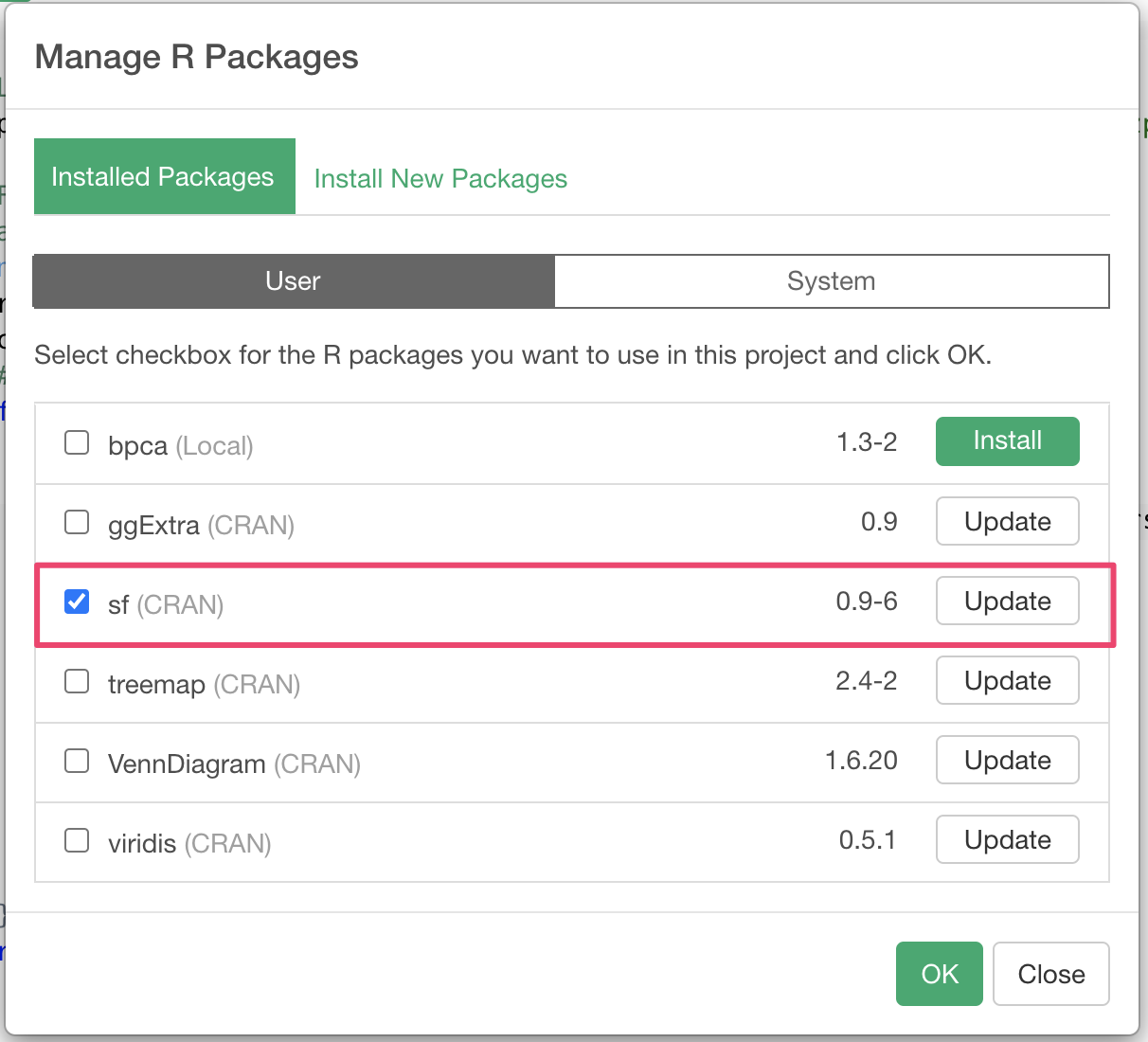
If you see the "sf" package in the installed package list, the installation is done and it is ready to use.
Import Data
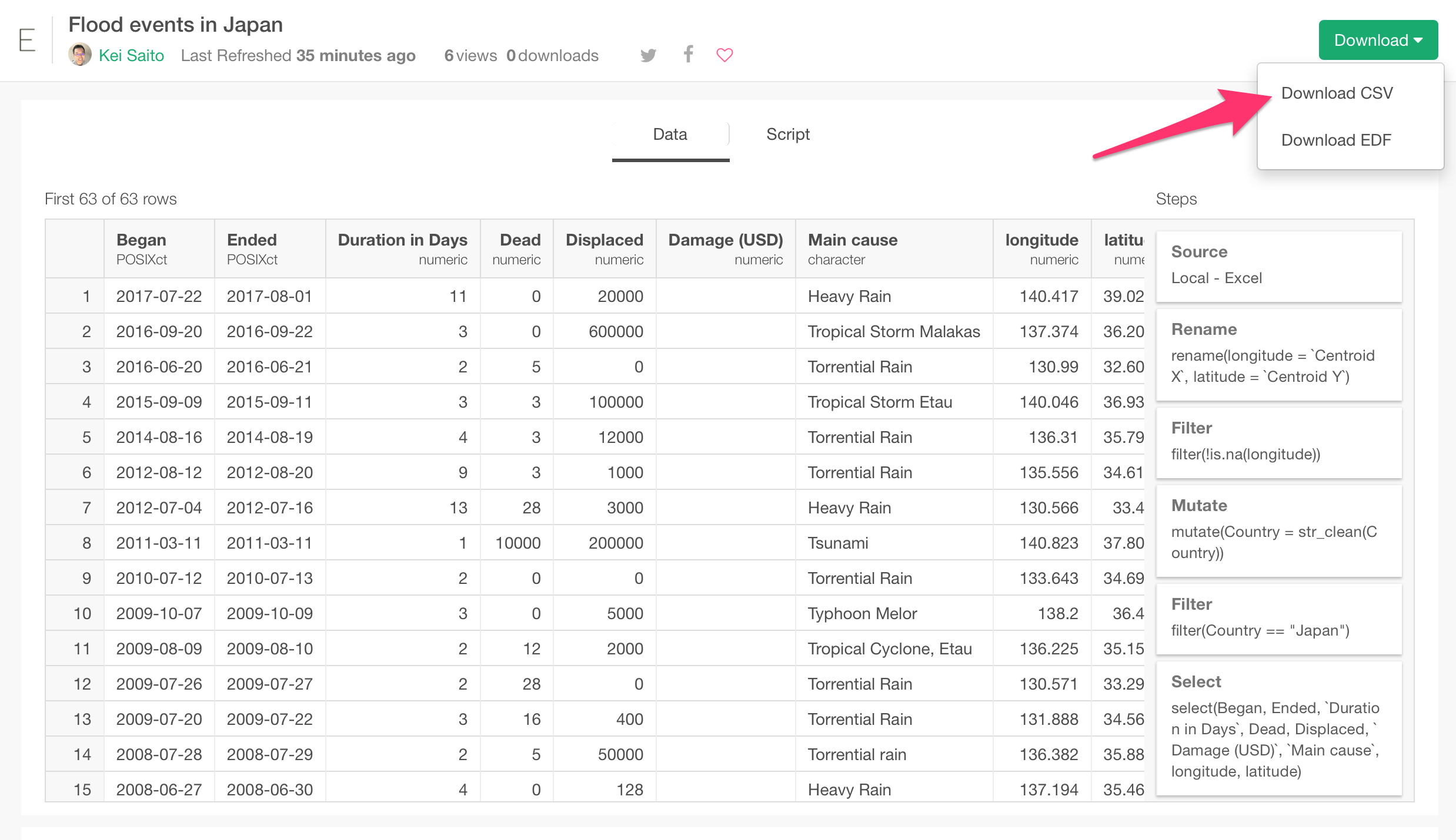
Here I prepared data about the major flood events in Japan since 1985. It is originally from Dartmouth Flood Observatory's Global Archive of Large Flood Events. You can visit here, and download the CSV data by choosing "Download CSV" menu.
Once you download the CSV data, go to Exploratory, open a project (or create a new project), click the ‘+’ icon next to the “Data Frames” and choose “File Data”.
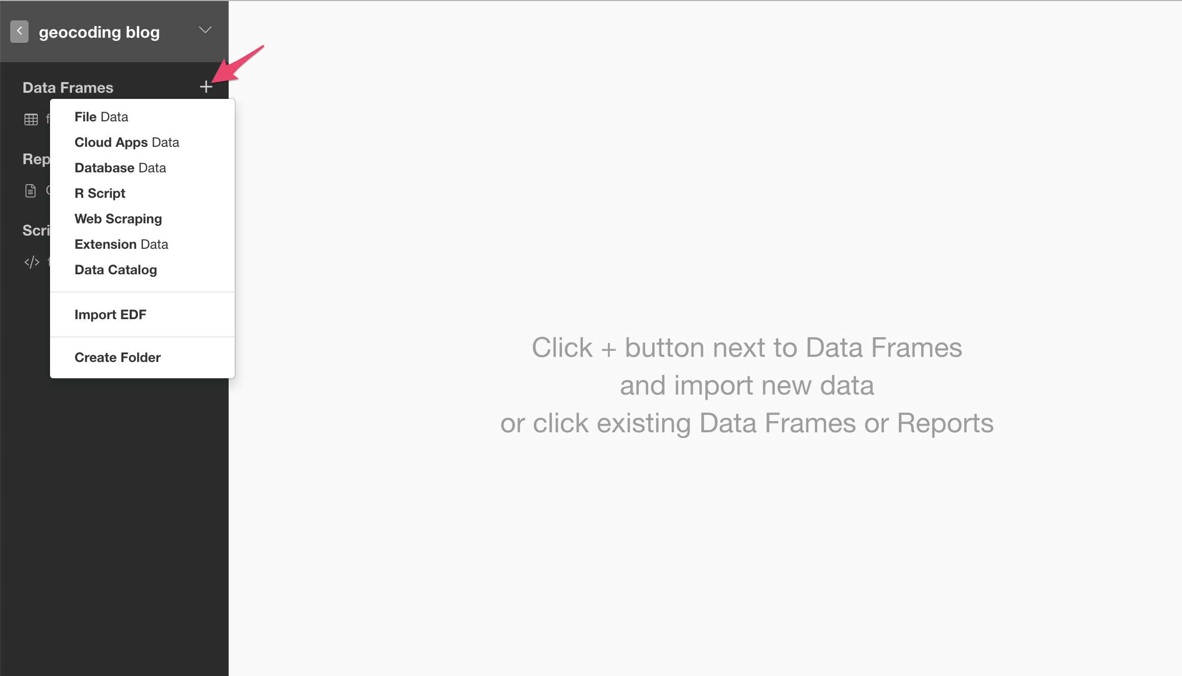
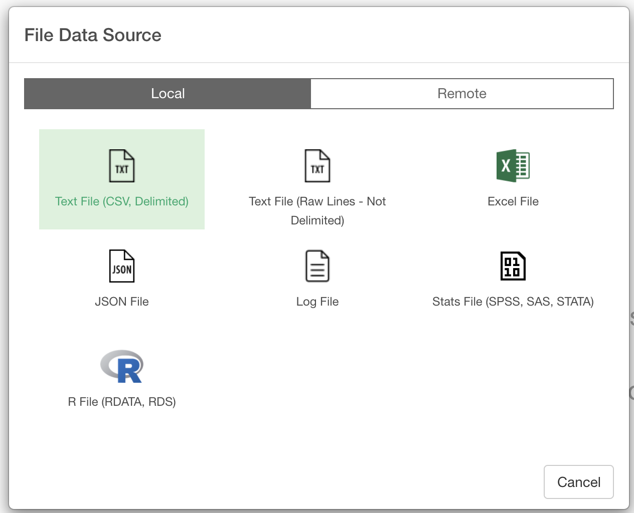
Then, it asks the file type. Click "Text File (CSV, Delimited)" and choose the file that you just downloaded.
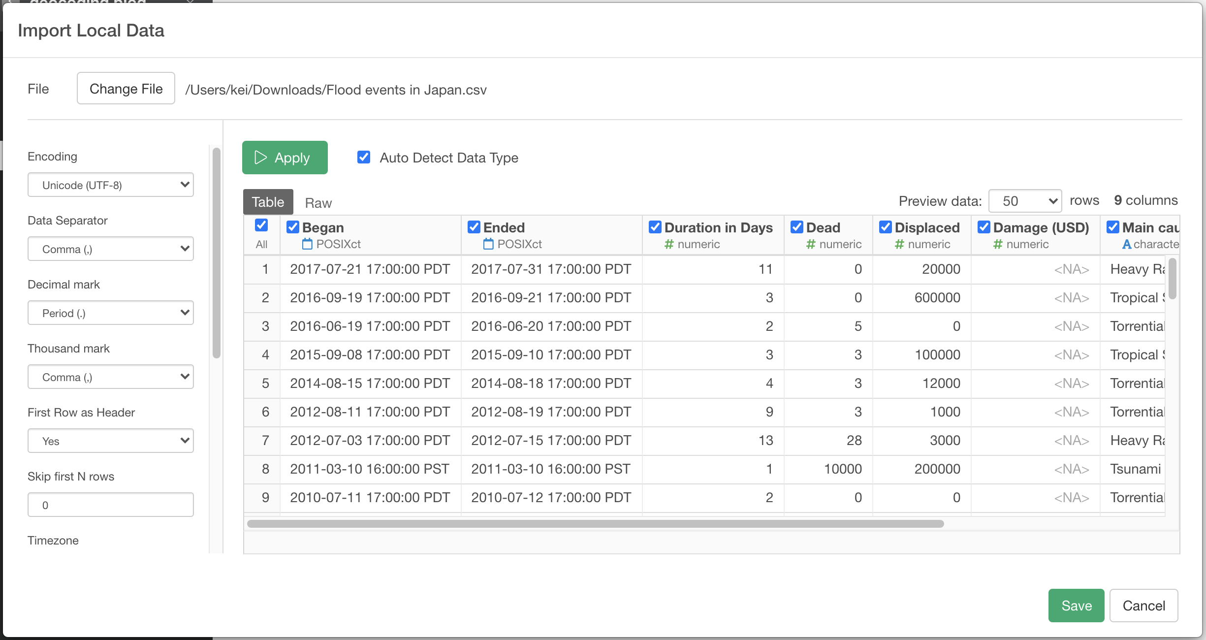
It will show the preview dialog. Click "Save".
Create a function to find location names from longitude/latitude data
Once you download and import the data to Exploratory, you can quickly check how the data looks like by clicking “Table” tab. Each row of the data represents a single flood event with date, damage, and where it happened with longitude/latitude data. But there’s no location name. Yes, we need location names like “Tokyo”.
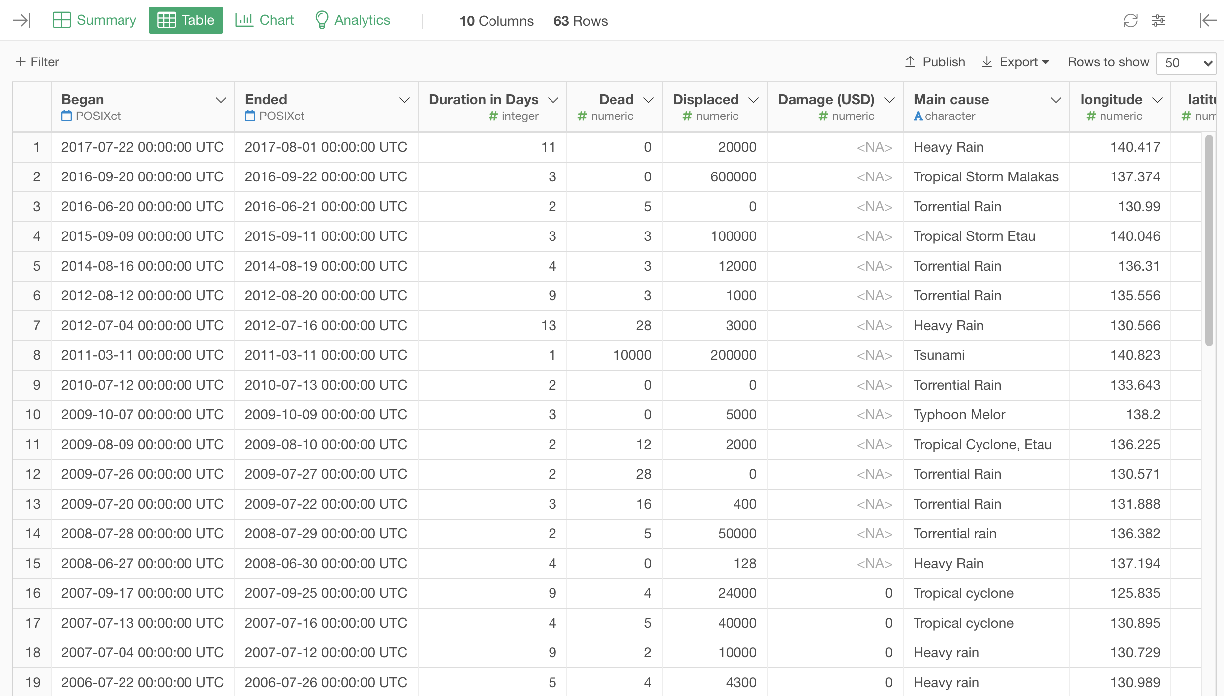
Ok, so here what I'm going to do is, creating a function, that takes longitude/latitude data and returns the prefecture names using Japan prefecture GeoJSON and sf package.
Click the "+" button right next to the "Script".
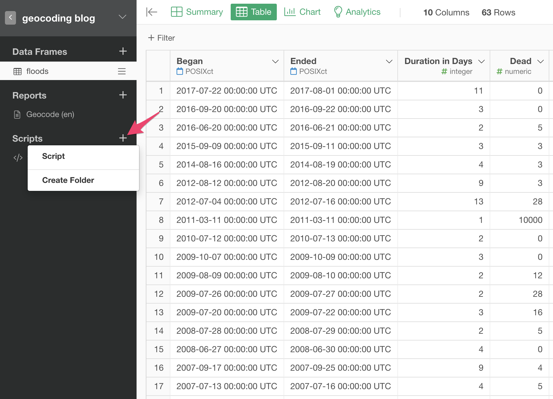
Give the name “find locations” to the script. Then it opens up the script editor window. Write an R script below, and click “Save” button on the upper right.
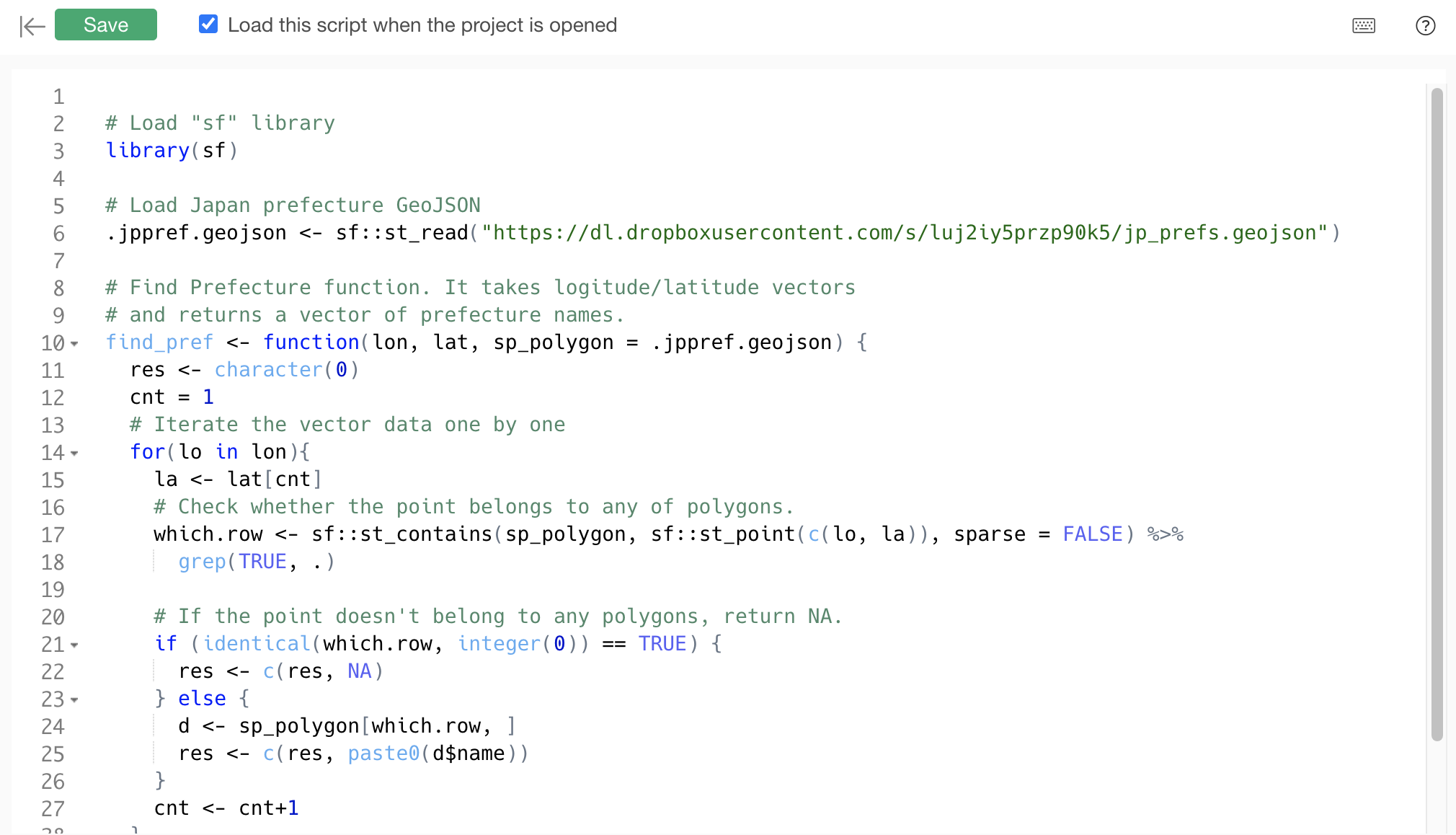
This script defines a function called “find_pref”. It takes longitude/latitude data and returns the prefecture names. It returns NA if the point doesn’t belong to any of the prefecture shapes.
# Load "sf" library
library(sf)

# Load Japan prefecture GeoJSON
.jppref.geojson <- sf::st_read("https://dl.dropboxusercontent.com/s/luj2iy5przp90k5/jp_prefs.geojson")

# Find Prefecture function. It takes logitude/latitude vectors
# and returns a vector of prefecture names.
find_pref <- function(lon, lat, sp_polygon = .jppref.geojson) {
  res <- character(0)
  cnt = 1
  # Iterate the vector data one by one
  for(lo in lon){
    la <- lat[cnt]
    # Check whether the point belongs to any of polygons.
    which.row <- sf::st_contains(sp_polygon, sf::st_point(c(lo, la)), sparse = FALSE) %>%
      grep(TRUE, .)

    # If the point doesn't belong to any polygons, return NA.
    if (identical(which.row, integer(0)) == TRUE) {
      res <- c(res, NA)
    } else {
      d <- sp_polygon[which.row, ]
      res <- c(res, paste0(d$name))
    }
    cnt <- cnt+1
  }
  return (res)
}
Using your own GeoJSON file
In this script, at line 6 (starting with “st_read”), I point to the GeoJSON of Prefectures in Japan by URL. If you want to use your own GeoJSON, you can change the URL to point to yours. If you don’t find any GeoJSON that you want to use, you can create one by yourself from Shapefile. You can read this article for more detail.
You also may need to change the script if you use your own GeoJSON file. The line you need to update is the line following.
res <- c(res, paste0(d$name))You need to update "name" to the property name defined in your GeoJSON file. For example, if your GeoJSON looks like the following;
{
  "type": "FeatureCollection",
  "features": [
    {
      "type": "Feature",
      "properties": {
        "GEO_ID": "0400000US04",
        "STATE": "04",
        "NAME": "Arizona",
        "LSAD": "",
        "CENSUSAREA": 113594.084
      },
      "geometry": {
        "type": "Polygon",
        "coordinates": [
          [
            [
              -112.538593,
              37.000674
            ],
            [
              -112.534545,
              37.000684
            ],
and you want to use "GEO_ID" property for the shape IDs, you want to update the line like the following.
res <- c(res, paste0(d$GEO_ID))Apply the function
Ok, everything is setup and ready. Now, this is the fun part, reverse geo-coding with GeoJSON!
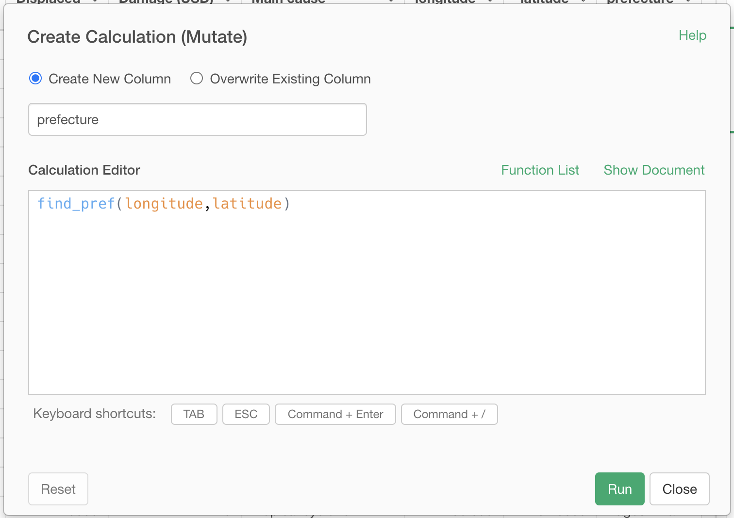
Click the data frame in the tree left-hand side to get back to the data frame, then click the column header menu of the "longitude" column and choose "Create Calculation (Mutate)".
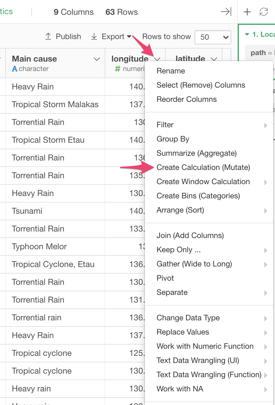
Choose "Create New Column", set "prefecture" to the New Column Name, and type in find_pref(longitude, latitude) at the Calculation. This means "Creating a new column with the name "prefecture" and it is based on the result of find_pref() function". Click "Run" button if it looks ok.
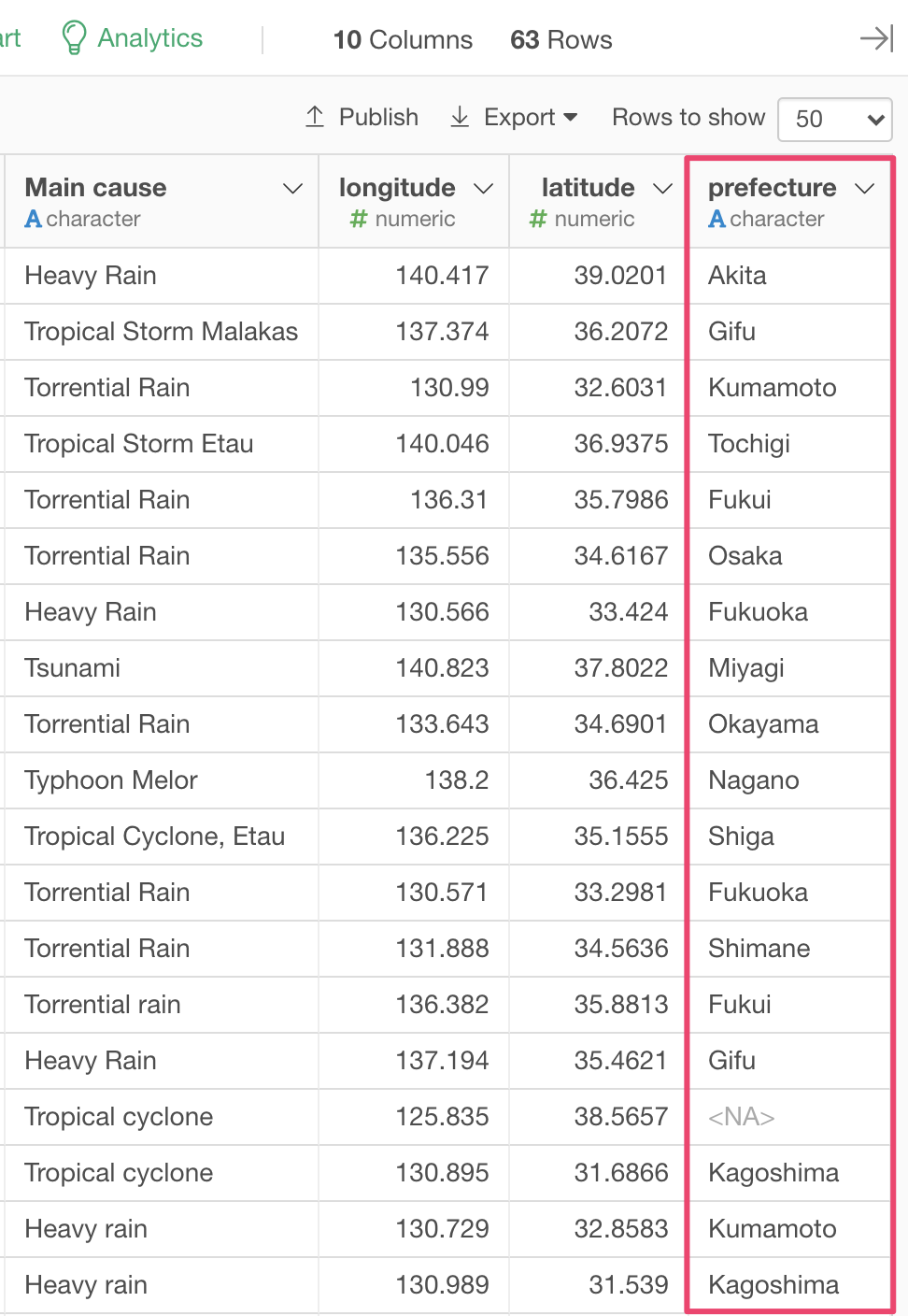
Then you see a new column "prefecture", and you see the prefecture names for each event.
Now, let's visualize it with Map.
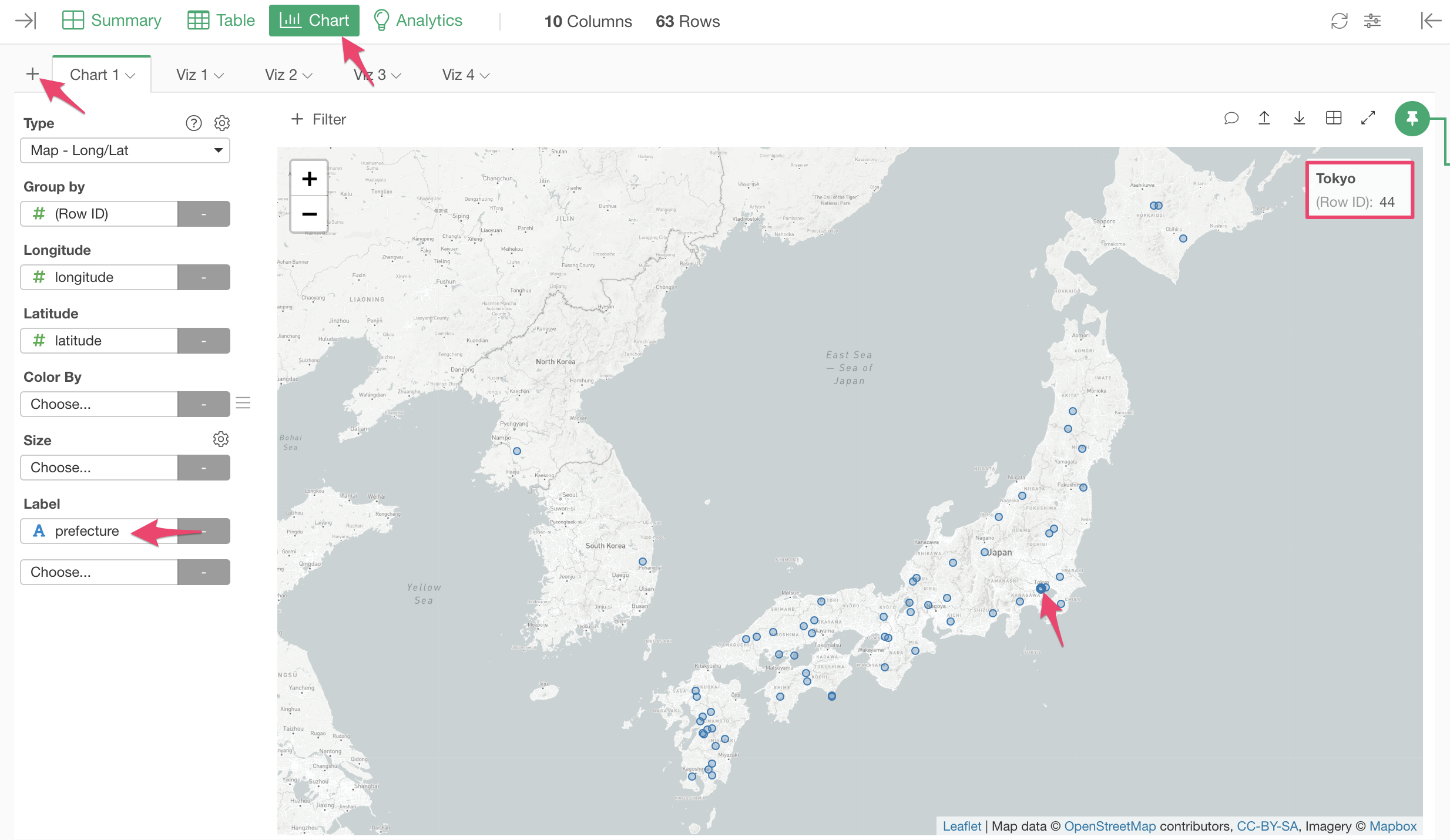
- Click the "Chart" tab
- Click the "+" button to create a new chart.
- Choose "Map - Long/Lat" for the type, it will automatically populate longitude and latitude columns and shows a map.
- Choose "prefecture" column that we just created above at the "Label".
Now you see the chart like the following. If you hover a dot, you see a prefecture name now.
Reverse Geocoding by using GeoJSON is a fast and standalone solution if you have an appropriate GeoJSON file on your local machine. But it has some limitations. For example, if you zoom in and hover the dot shown in the screenshot below, you don’t see the location name.
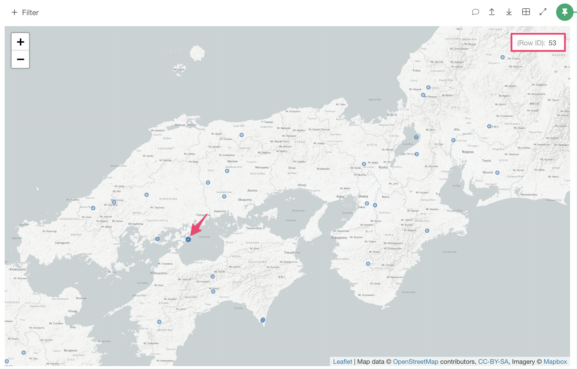
This is because this location doesn't belong to any of the GeoJSON shapes. Here I use the simplified version of the Japan GeoJSON for reducing the file size. The simplifying process is to use fewer lines for each shape, so it loses the detailed cost line information. I can use higher resolution GeoJSON to cover such locations, but it will make the reverse-geocoding operation slower because the file size will be larger.
This is when you want to consider using geocoding services like Google MAP API, which I’m going to talk about in the next post. Stay tuned!
This analysis is done by Exploratory, the modern data science tool for non-programmers. If you are interested in, sign up from here for a free trial. If you are a student or teacher it’s free!
R Packages used in this post