Prediction Models
During this tutorial we will explore a complex dataset and use it to predict student droput. The main goals of this tutorial are to:
- Manipulating complex interlinked datasets
- Format the data in a format that is accepted by statistical and machine learning models
- Use statistical models for prediction
- Use machine learning models for prediction
- Evaluate prediction certainty
- Visualize prediciton
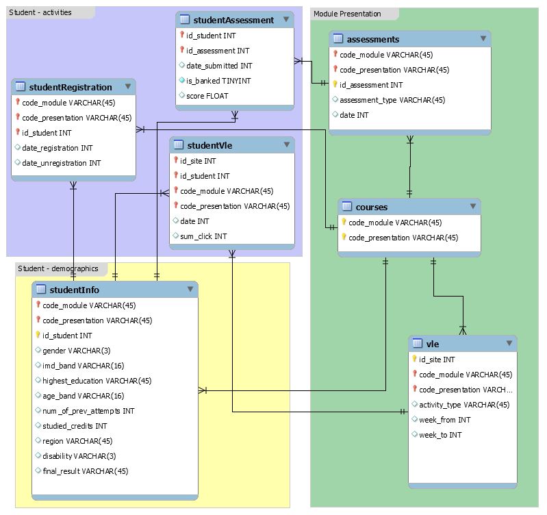
This dataset is reduced verison of the one available in https://analyse.kmi.open.ac.uk/open_dataset and correspond to student activity in several MOOCs of the Open University UK.
Step 1: Loading the Data
First we will import the csv files with the data:
courses.csv
File contains the list of all available modules and their presentations. The columns are:
- code_module – code name of the module, which serves as the identifier.
- code_presentation – code name of the presentation. It consists of the year and “B” for the presentation starting in February and “J” for the presentation starting in October.
- length - length of the module-presentation in days.
The structure of B and J presentations may differ and therefore it is good practice to analyse the B and J presentations separately. Nevertheless, for some presentations the corresponding previous B/J presentation do not exist and therefore the J presentation must be used to inform the B presentation or vice versa. In the dataset this is the case of CCC, EEE and GGG modules.
assessments.csv
This file contains information about assessments in module-presentations. Usually, every presentation has a number of assessments followed by the final exam. CSV contains columns:
- code_module – identification code of the module, to which the assessment belongs.
- code_presentation - identification code of the presentation, to which the assessment belongs.
- id_assessment – identification number of the assessment.
- assessment_type – type of assessment. Three types of assessments exist: Tutor Marked Assessment (TMA), Computer Marked Assessment (CMA) and Final Exam (Exam).
- date – information about the final submission date of the assessment calculated as the number of days since the start of the module-presentation. The starting date of the presentation has number 0 (zero).
- weight - weight of the assessment in %. Typically, Exams are treated separately and have the weight 100%; the sum of all other assessments is 100%.
If the information about the final exam date is missing, it is at the end of the last presentation week.
vle.csv
The csv file contains information about the available materials in the VLE. Typically these are html pages, pdf files, etc. Students have access to these materials online and their interactions with the materials are recorded. The vle.csv file contains the following columns:
- id_site – an identification number of the material.
- code_module – an identification code for module.
- code_presentation - the identification code of presentation.
- activity_type – the role associated with the module material.
- week_from – the week from which the material is planned to be used.
- week_to – week until which the material is planned to be used.
studentInfo.csv
This file contains demographic information about the students together with their results. File contains the following columns: - code_module – an identification code for a module on which the student is registered. - code_presentation - the identification code of the presentation during which the student is registered on the module. - id_student – a unique identification number for the student. - gender – the student’s gender. - region – identifies the geographic region, where the student lived while taking the module-presentation. - highest_education – highest student education level on entry to the module presentation. - imd_band – specifies the Index of Multiple Depravation band of the place where the student lived during the module-presentation. - age_band – band of the student’s age. - num_of_prev_attempts – the number times the student has attempted this module. - studied_credits – the total number of credits for the modules the student is currently studying. - disability – indicates whether the student has declared a disability. - final_result – student’s final result in the module-presentation.
studentRegistration.csv
This file contains information about the time when the student registered for the module presentation. For students who unregistered the date of unregistration is also recorded. File contains five columns: - code_module – an identification code for a module. - code_presentation - the identification code of the presentation. - id_student – a unique identification number for the student. - date_registration – the date of student’s registration on the module presentation, this is the number of days measured relative to the start of the module-presentation (e.g. the negative value -30 means that the student registered to module presentation 30 days before it started). date_unregistration – date of student unregistration from the module presentation, this is the number of days measured relative to the start of the module-presentation. Students, who completed the course have this field empty. Students who unregistered have Withdrawal as the value of the final_result column in the studentInfo.csv file.
studentAssessment.csv
This file contains the results of students’ assessments. If the student does not submit the assessment, no result is recorded. The final exam submissions is missing, if the result of the assessments is not stored in the system. This file contains the following columns: - id_assessment – the identification number of the assessment. - id_student – a unique identification number for the student. - date_submitted – the date of student submission, measured as the number of days since the start of the module presentation. - is_banked – a status flag indicating that the assessment result has been transferred from a previous presentation. - score – the student’s score in this assessment. The range is from 0 to 100. The score lower than 40 is interpreted as Fail. The marks are in the range from 0 to 100.
studentVle_reduced.csv
The studentVle.csv file contains information about each student’s interactions with the materials in the VLE. This file contains the following columns: - code_module – an identification code for a module. - code_presentation - the identification code of the module presentation. - id_student – a unique identification number for the student. - id_site - an identification number for the VLE material. - date – the date of student’s interaction with the material measured as the number of days since the start of the module-presentation. - sum_click – the number of times a student interacts with the material in that day.
Step 2: Extracting Outcomes and Predictors
Outcomes
Due to the size of the dataset, we will only work with one of the MOOCs, the moudule "DDD".
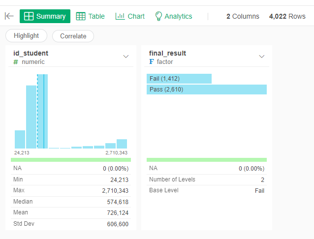
First we calculate the outcome of the students from the different tables. This information is the final status (Pass, Fail), if the student has withdrawn (dropout) and the final score in the course.
Final State (Pass/Fail)
First, get the final state (Pass, Fail) of the students in a given course. If the student has a "Withdrawn" state, we remove them from the list. If the student has "Distinction" as a final state, we count it as a "Pass".
- Go to the studentInfo dataset
- Branch the dataset to a new one called "final_state"
- Move to the new "final_state" dataset
- Filter only records in which code_module is "DDD"
- Filter out those records which final_result is "Withdrawn"
- We change the value of the variable final_result so "Distinction" is converted into "Pass" (Replace Values -> New Values)
- Convert final_result to Factor
- Select only the "id_student" and "final_result" columns
Dropout
Next, to obtain the if a student has droped-out of the course we use the fina_result variable. Dropout students are marked with a "Withdrawn".
- Go to the studentInfo dataset
- Branch the dataset to a new one called "dropout"
- Go to the new dropout dataset
- Filter only records in which code_module is "DDD"
- Change the value of the variable final_result. Where it has Withdrawn, replace with "Dropout", all else, replace with "No dropout"
- Convert final_result into a Factor
- Change the name of final_result column to dropout
- Select only the id_student and dropout columns

Final Grade
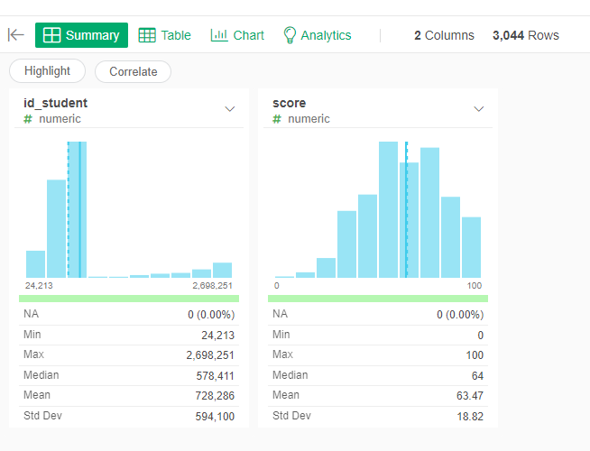
Continuing, we will obtain the final grade of the student, given the course. This is a little more complicated because we need to use two datasets. First, we need to find what is the ID code of the “Exam” assessment from the “assessments” dataset for the course. Then we need to use those ID codes to select only those assessments from the “studentAssessment” dataset.
- Go to the assessments dataset
- Branch the dataset to a new one called "final_grade"
- Go to the new "final_grade"
- Filter only records in which code_module is "DDD"
- Filter only records in which the assessment_type is "Exam"
- Do a Left Join with studentAssessment dataset where the "id_assessment" is the same.
- Select only the id_student and score columns
Predictors
Next that will extract the predictors, we should specify not only the course from which we want the information ("DDD"), but the period of time since the start of the course at which want to make the prediction (50 days since the start of the course).
Assessment delivered and average score
We will start with the information about the assessments deliverd by the student. We will extract two predictors, the average grade of the assessments present until that date, and the total number of assessments presented.
- Go to the assessments dataset
- Branch a new dataset and name it "student_results"
- Go to the new dataset
- Filter only records from the course "DDD"
- Filter only records in which date is less than "50"
- Do a Left Join with studentAssessments dataset by id_assessment
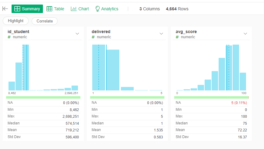
- Summarize, grouping by "id_student" and the values will be the score (average) and the Number of Rows (that is the number of assessemnts took by the student)
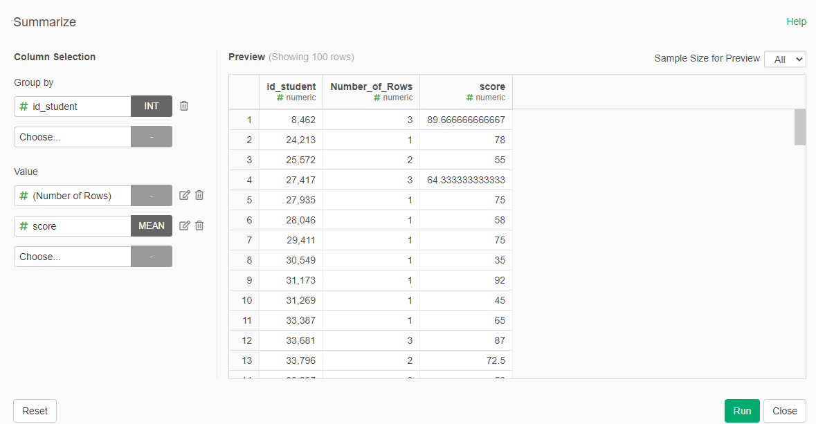
- Change the name of the colum "Number_of_Rows" by "delivered" and the "score" by "avg_score"
Lateness
Then we obtain the information about lateness delivery of assessments. For this we need information about the deadline of the assessment and we substract the deliver day to calculate if it was delivered late.
- Go to the assessment dataset
- Branch a new dataset called "late_assessments"
- Filter just the course "DDD"
- Filter the date for less than 50 days
- Left join with studentAssessements by "id_assessment"
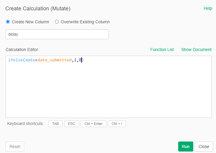
Create a calculation (mutate) a new column called "delay" with the formula ifelse(date<date_submitted,1,0)
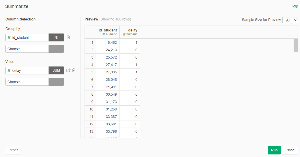
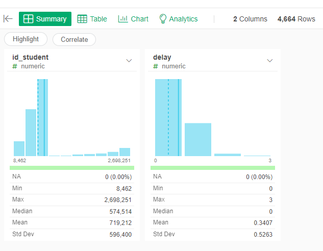
- Summarize grouping by id_student and as value use the sum of delay
Rename the delay column to "sum_delays"
Clicks on the LMS
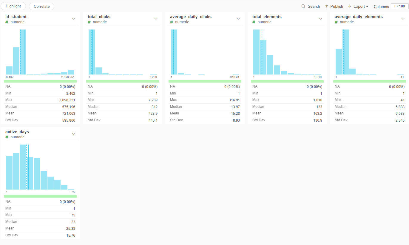
Finally we will get information from the number of clicks in the VLE information. We will get tree predictors, the total number of clicks, the average number of clicks per day and the number of active days.
- Go to the studentVle_reduced dataset
- Branch a new dataset called "click_info"
- Go to the new dataset
- Filter the course to just "DDD"
- Filter the records in which date is less than 50
- Summarize grouping by id_student and date, the value should be sum_clicks (sum) and Number of Rows
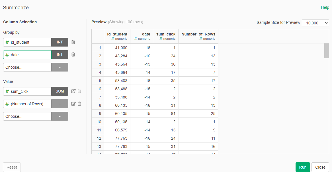
- Rename the colum sum_clicks to daily_clicks, and Number_of_Rows to daily_elements
- Summarize again, by id_student. The values are daily_clicks (sum), daily_clicks (avg), daily_elements (sum), daily_elements (avg), and Number of Rows
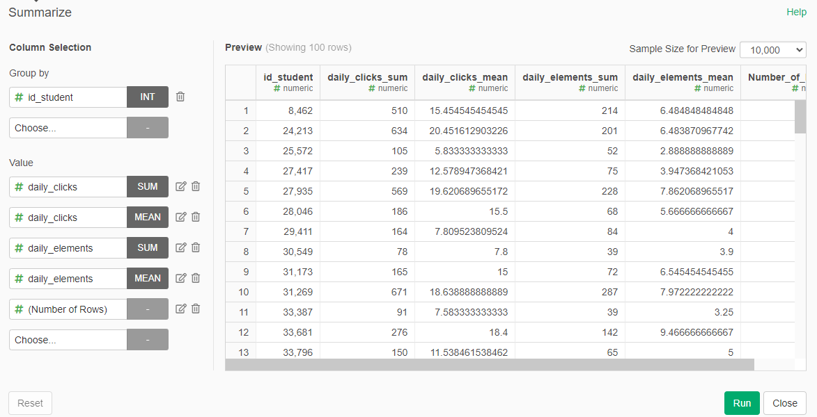
- Rename the columsn daily_clicks_sum to total_clicks, daily_clicks_avg to average_daily_clicks, daily_elements_sum to total_elements, daily_elements_avg to average_daily_elements, and Number of Rows to active_days
General student information
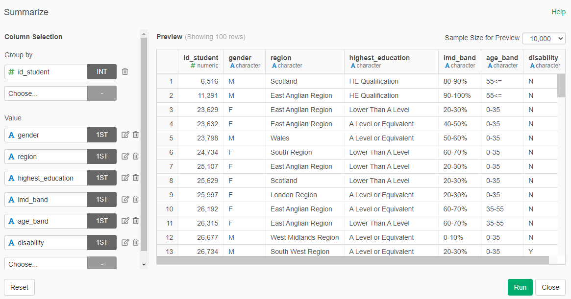
We generate a dataset that contain additional information about students
- Go to the studnetInfo dataset
- Branch it into a new dataset called "student_general_info"
- Go to the new dataset
- Filter the course to just "DDD"
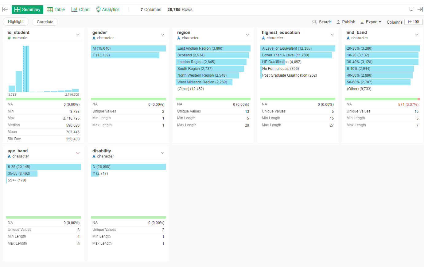
- Select only the columns: id_student, gender, highest_education, imd_band, age_band, and disability
- Summarize by id_student, for all variables (gender, region, highest_education, imd_band, age_band, and disability) select the first value
Step 3: Assembling the Predictors
First we will put together the extracted numerical predictors for the given course ("DDD") and cut-off days (50).
- Go to students_results dataset
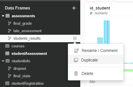
- Duplicate the dataset (after the last step) and change its name to "predictors"
- Go to the predictors dataset
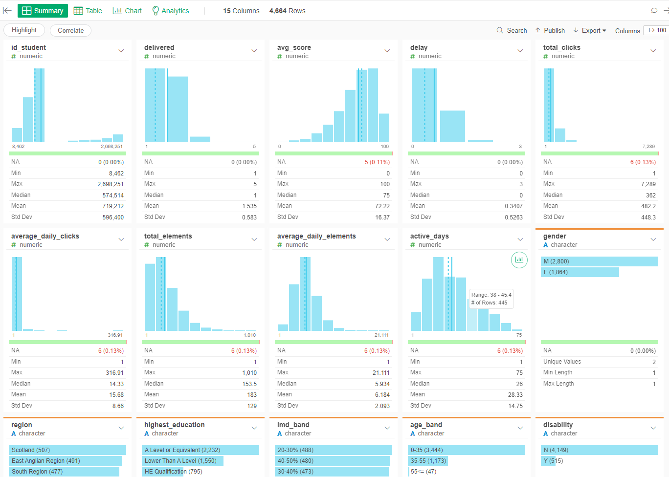
- Left join with the late_assessment dataset by id_student
- Left join with the click_info dataset by id_student
- Left join with student_general_info dataset by id_student
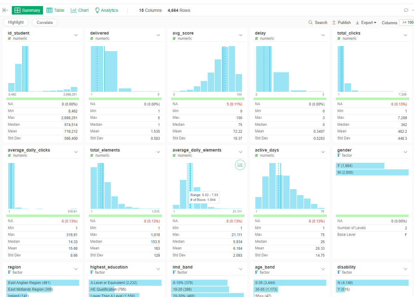
- Convert those predictors that should be factors into factors
Step 4: Assembling the Outcomes
Now, we create the outcome values of Pass/Fail (finalState), the final grade (finalGrade) and the dropout (dropout)
- Go to predictors and duplicate the dataset into one called complete_info
- Go to complete_info dataset
- Left join with the final_state dataset by student_id
- Left join with the droput dataset by student_id
- Left join with the final_grade dataset by student_id
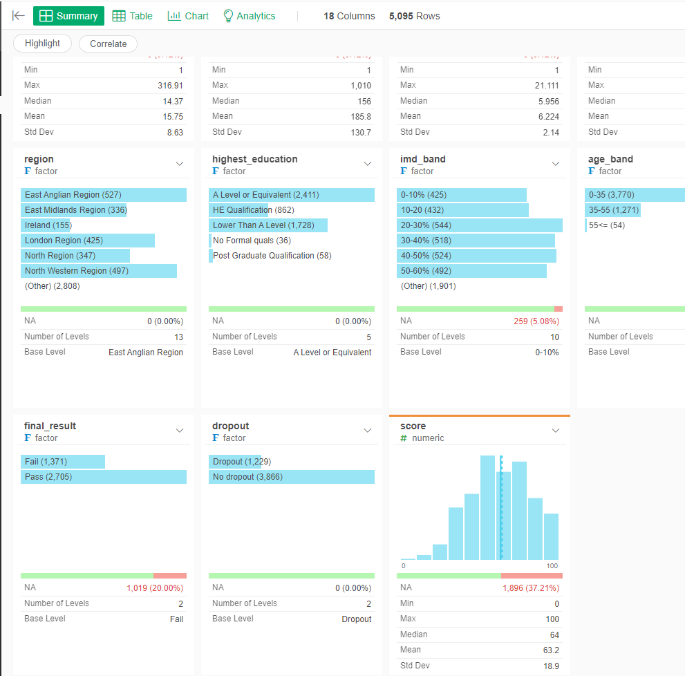
Step 5: Classification models
We will build classification models to predict if a student will pass or fail the course and another to determine if the students will dropout of the "DDD" course.
Decision Tree Classificator for Passing
We will start with the simplies classificator, the decision tree.
- Go to the complete_info dataset
- Go to Analytics and create a new one
- Select the Type "Decision Tree"
- In Target variable select "final_result"
- In predictive variables select: delivered, avg_score, delay, total_clicks, average_daily_clicks, total_elements, average_daily_elements, active_days, gender, region, highest_education, imd_band, age_band, and disability
- Go to the gear besides type
- Go to the bottom and select TestMode as TRUE and Ratio for Test Data as 0.3. In this way a test set with 30% of the data will be created.
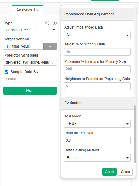
- Run the analytic
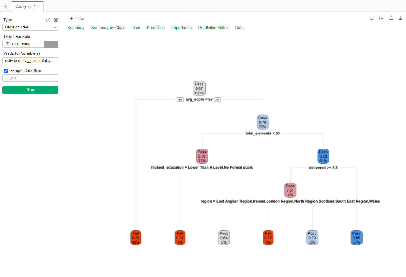
The result tell us that if, in the first 50 days of the course you have an average score higher than 67, you visited more than 85 elements in the LMS and delivered less than 2.5 assessments you have a 85% chance of passing the course (57% of the population comply with this characteristics). On the other hand if your average score is less than 67 in the first 50 days, you only have a 0.36 of Passing (28% of the training set was in this situation).
If we want to know how accurate is the model, go to the Prediction Matrix (confusion matrix).
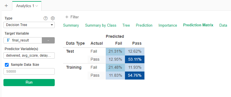
We see than in the test set, 21.31% failed the course, and the model predicted that they will fail. Also, in the test set, 53.11% passed the course, and the model predicted that they will pass. In total, the model is 21.31+53.11 (74%) accurate, that is, it fails for around a quarter of the cases. Not good, not bad.
If you want to see all the metrics for the model, go to Summary.  Here we can see that the performance in the test and training sets are similar, indicating a consistent model that is not overtrained on the training data. The accuracy rate is the one that we have calculated before (76% for the training set, 74% for the test set).
We can also see which variables are more important to determine if you will pass or fail. Go to Importance tab:
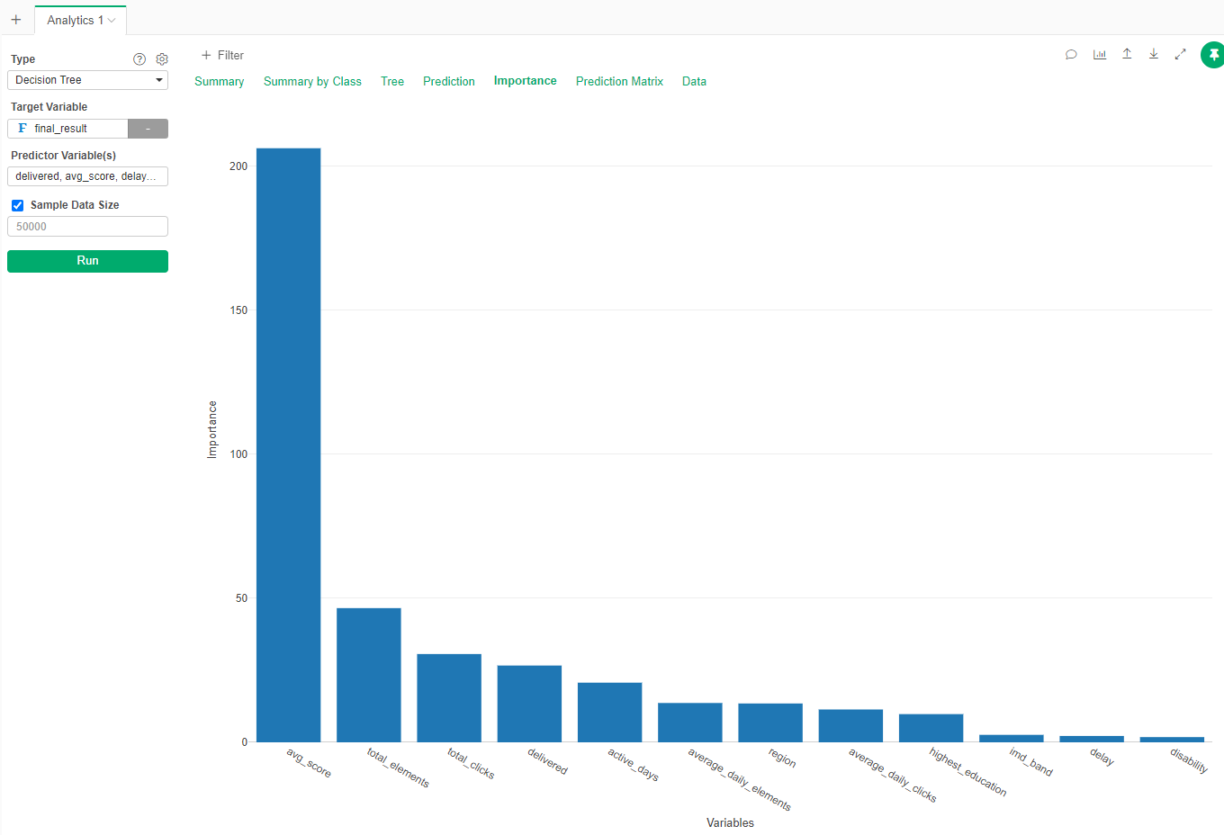
We can see that your score in the first 50 days is highly predictive of your passing or failing, while your disability status is not so much.
Decision Tree for Dropout
Now we will create a decision tree for the dropout.
- Duplicate the complete_info dataset into a dropout_info set
- Create an Decision Tree with the same predictor variables, but with dropout as target. Do not forget to create the Training and Test sets in the Gear beside the type of analytic.
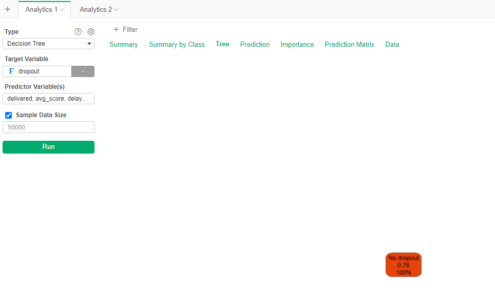
!!! No tree !!!
If you go to the Prediction Matrix you see why, it is basically assigning No dropout to all the students (and still being 75% accurate).
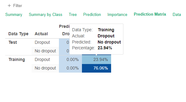
This is due to the fact that very few students dropout compared to the whole population. The algorihtm provided by Exploratory has a way to balance the samples.
- Go to the Gear and seach for Imbalanced Data Adjustment and in Adjust Imbalanced Data select "Yes"
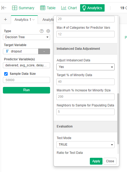
Now you will have something like this:
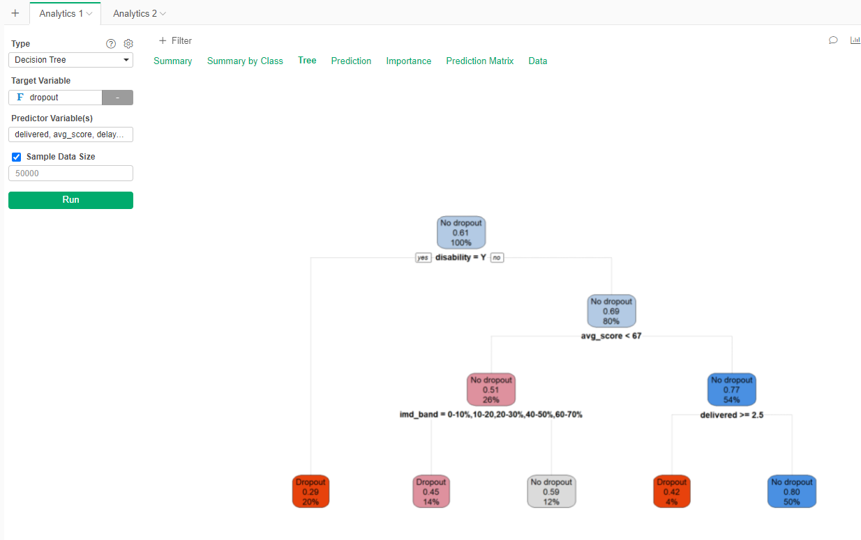
Now we see that disability, while not important to pass or fail the course, it is actually important to being able to finish the course.
The prediction matrix tell us that there are errors, but they stay below the 30% for the test set.
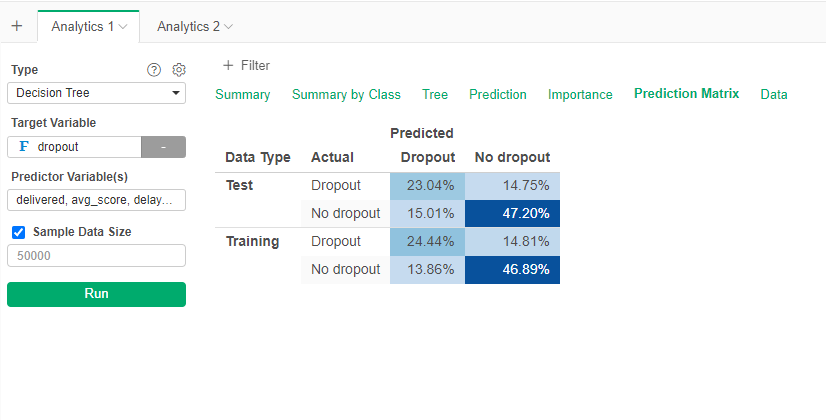
This model is a little less accurate with a 70% accuracy:

Logistic Regression for Passing / Failing
Let's try a statistical method for classification, Logistic Regression. This method only work for TRUE/FALSE variables, so we need to convert the Pass/Fail factor variable to a logical variable.
- Go to the final_result_data dataset
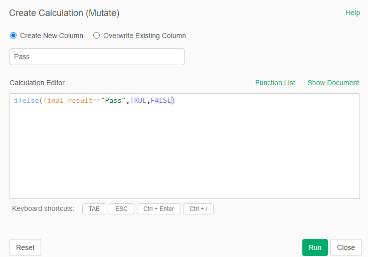
- Create a calculation (mutate) to create a new column "Pass" with the following formula: ifelse(final_result=="Pass",TRUE,FALSE)
- Go to Analytics and create a new one
- Select type "Logistic Regression"
- Select the target variable "Pass"
- Select the ones used previously as predictors
- Go to the Gear and select 30% Test set
- Run
- Go to the Prediction Matrix tab
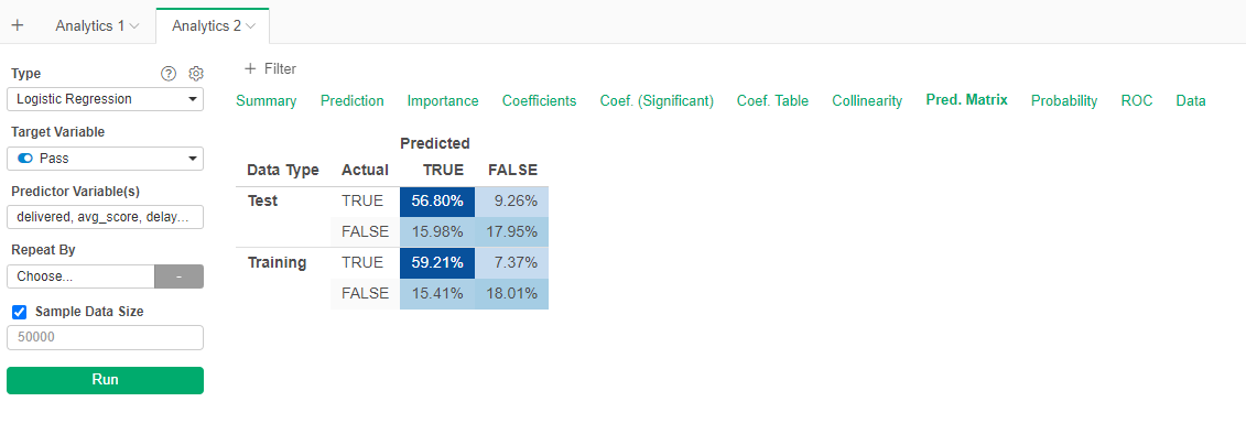
We can see that the performance is similar to the decision tree, however there are more Type II errors and less Type I errors. The summary tell us that the model is 75% accurate. Just 1% more than the decison tree.
The model also let us know what are the important varibles (avg_score and active_days). 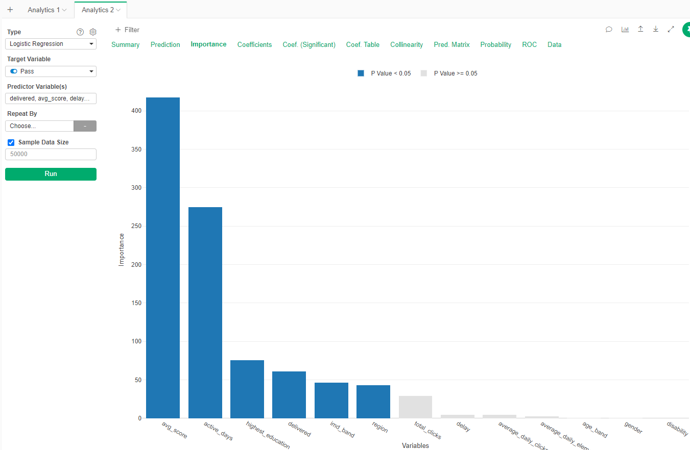
Logistic Regression for Dropout
Now we apply this algorithm to the dropout data. Again, we need to create a logical variable out of the dropout information.
- Go to the dropout_info dataset
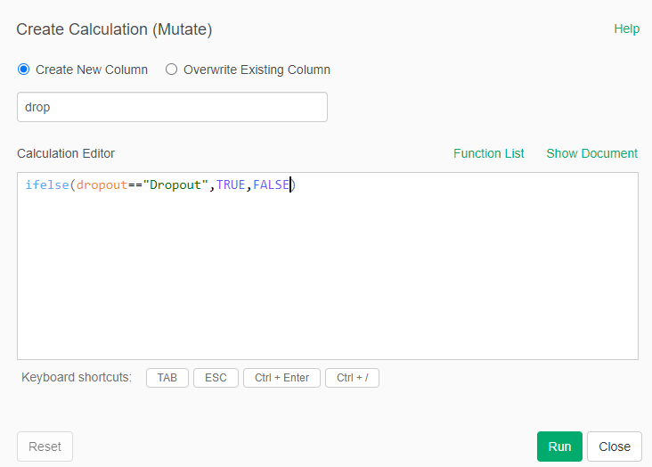
- Create a new calculation (mutate) for a new column called drop with the following formula: ifelse(droput=="Dropout",TRUE,FALSE)

Now lets train the model:
- Go to Analytics
- Create a new analytics type "Logistic Regression"
- Select the drop variable as target
- Select the predictor variables
- Go to the Gear and select 30% of test data
- Run
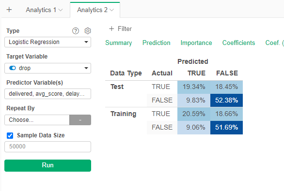
Something similar is happening. Most people is classified as FALSE. Let's balance
- Go to the Gear and select Adjust Imbalanced Data (yes)
- Run
Now the model behave much better. Again disability and avg_score seem to be the most important variables to predict dropout. This model it is a little bit more accurate (72%) than the decision tree.
Random Forest for Pass/Fail
Now we will run the Random Forest algorithm over the same data
- Go to the final_result_data dataset
- Add a new Analytics
- Type Random Forest
- Select final_result as target variable
- Add the predictor variables
- In the Gear select 30% test set
- Run
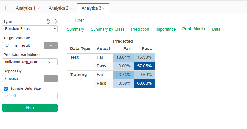
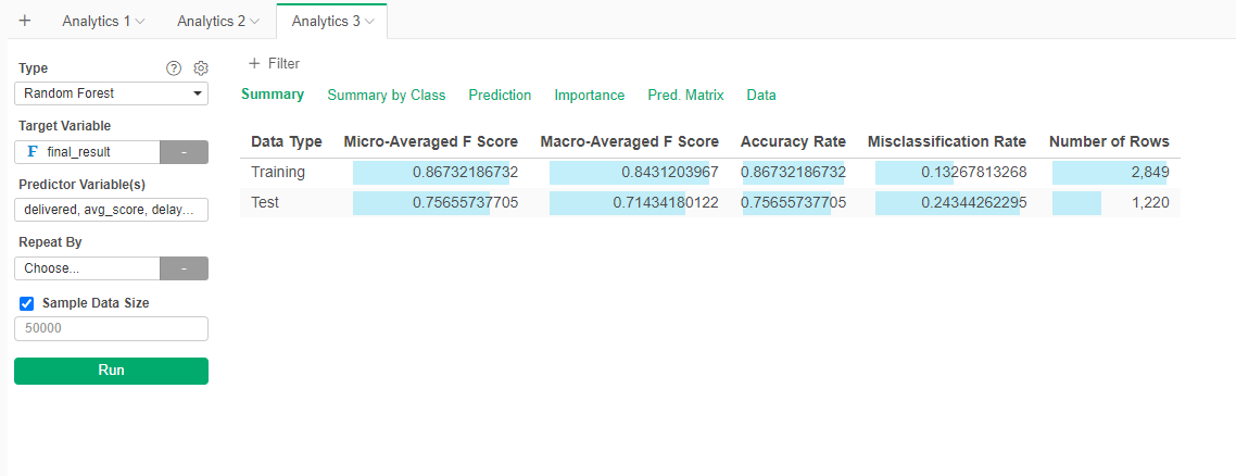
The results seem better. However, a look at the summary tell us that the accuracy is just marginally better (76%).
Average score and total elements used seem to be the main variables.
Random Forest for Dropout
Now we apply Random Forest to the dropout data.
- You know what to do. Do not forget to balance the data.
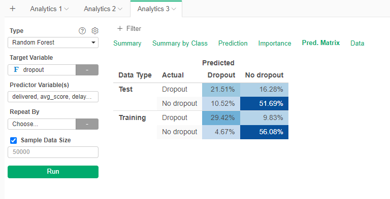
It seems that we have slight better performance. The summary says that the model is 73% accurate in the test set.
As we can see all the models have a similar performance, the inacurracy if due mainly to some missing information.
Step 6: Regression Models
We will now will try to predict the final grade of the students.
Linear Regression
- Go to the complete_info dataset and duplicate it into "final_grade_data"
- Go to the new dataset
- Create a new Analytic: Linear Regression
- Set the target variable to "score"
- Set the predictor variables
- Go go the Gear and select 30% test set
- Run
- Go to Summary

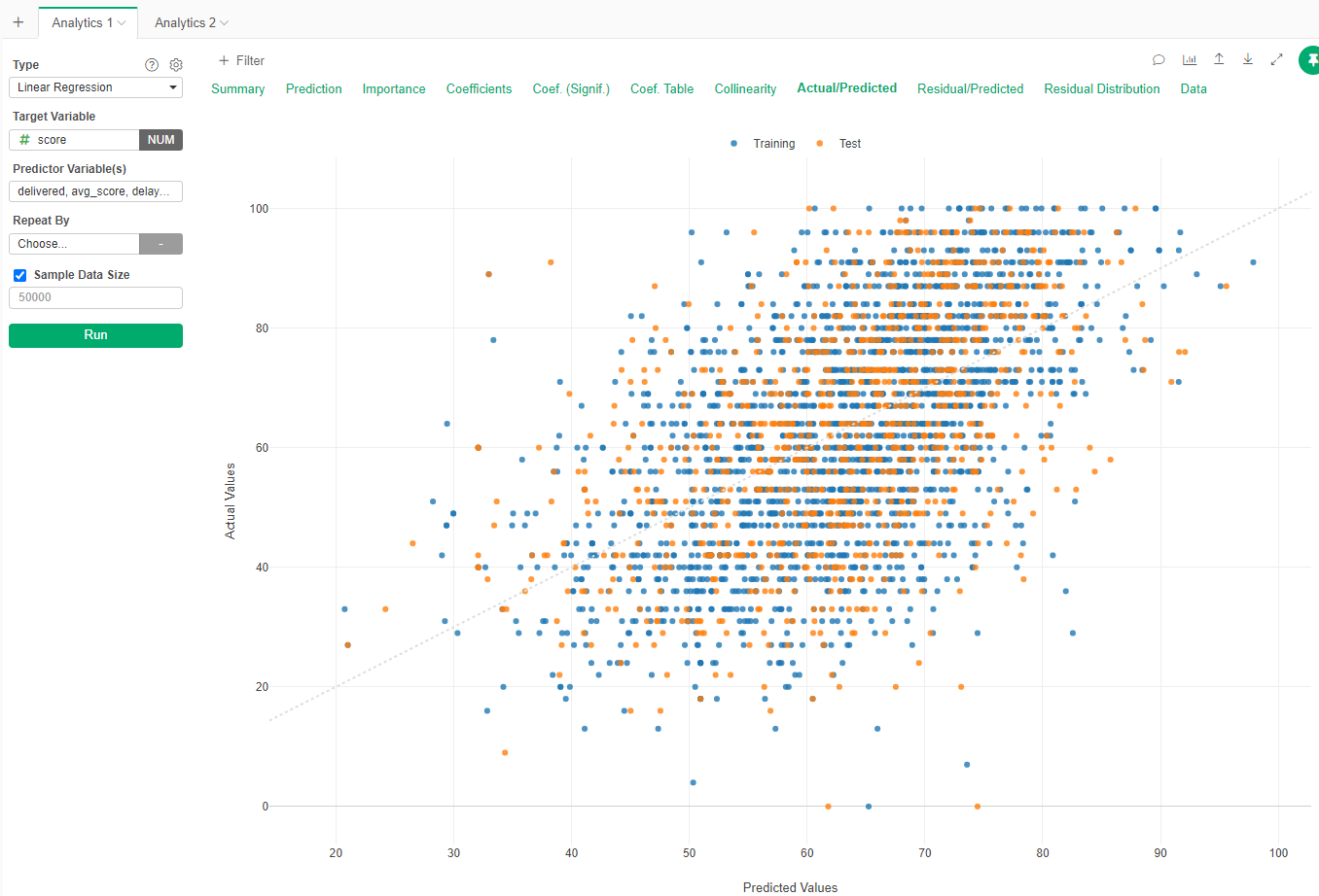
We can see that the model is not good at predicting actual grade. The R Square is low (0.26), that means that the variables cannot explain the variability in scores. The error is high +/- 16.24 points in average (RMSE).
If you go to Actual/Predicted the graph is not a clear line (as you would expect from a good prediction)
Random Forests
Now we will apply Random Forest as a regression algorithm
- You know the steps. Do not forget to add the test set.
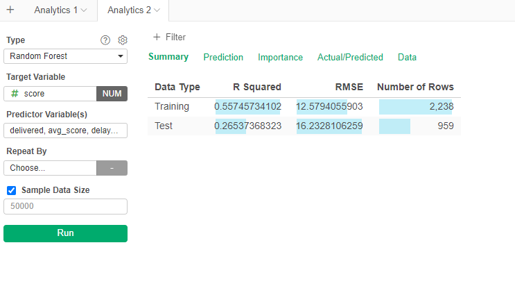
The R Squared is still low (0.26), meaning that the variables are not able to explain the variability of the score.
If we go to importance, we see that avg_score is the main variable to predict the final score.
Step 7: Report
Create a Report comparing the performance of the different models and which one will you choose and why.