Clustering of Students
Welcome to the Clustering turorial! In this analysis we are going to look at data collected by the lead instructor of a first year chemistry course at a mid-sized state university in the northeastern US. The course is a required for all science majors and consistently has an enrollment of around 100-120 students. The main learning objectives of the course relate to knowledge of core chemistry concepts and manipulation of chemical equations. It is a class that students often struggle with, particularly if they do not have strong prior preparation from high school.
In 2018, the instructor gave students a short quiz in the first week of the class with questions on each of the two key areas to assess their incoming knowledge about chemistry concepts and ability to work with chemical equations; she gave another quiz in the third week on the concepts and equations covered in the first two weeks of the semester to see how, if at all, the students were improving.
We will perform a cluster analysis on this data to see if we can identify profiles of common student types. This information could be useful to help the instructor better understand the class and how to support them. We will first need to clean and tidy the data to get it ready for analysis (though actually this data comes to us in pretty good shape) and then we will be performing a cluster analysis to see if we can identify some number of "groups" (clusters) of students who have similar patterns of data.
Loading and Understanding the Data
Load the data (CSV format):
- The file is named conceptsequationswk1and3allstudents.csv and you can download it here.
Take a look at the data and think about
How many cases are there and what do they represent?
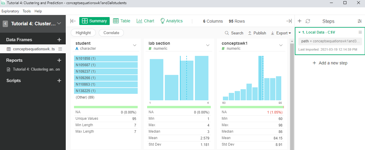
- See the number of rows, there are 95 cases. Each case seems to represent 1 student.
- How many variables are there and what does each one represents?
- There are 6 columns that seem to represent 6 different variables: the ID of the student (student), the section they belong (lab section), the scores for the weekly concept quizzes (conceptswk1, conceptswk3) and the scores in the equations quizzes (equationswk1, equationswk3)
- Do you notice any potential problems in the data and if so, what might have caused them?
- There are 5 null values in the database. These null values belong to 3 students. Student N276373 has null values in “conceptswk1” and “equationswk1”. Student N947943 has null values in “conceptswk3” and “equationswk3”. These two student probably didn’t attend one of the quizzes. Student N505894 has a null value in “equationswk3”. This student probably didn’t answer any questions regarding chemistry equations in week 3’s quiz. Another explanation of the null values is that there was a data entry mistake. Furthermore, “lab section” should be a factor data instead of numeric data.
Examining the Data Distribution
Review the histograms of the variables in the Summary view
Identify clear data entry errors
- There not seem to be any error apart from the missing values.
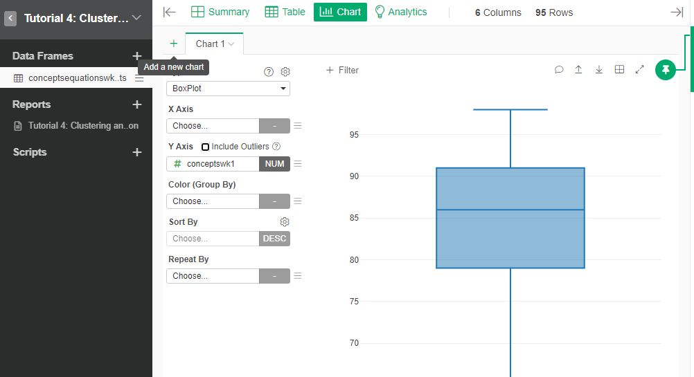
Identify potential outliers
- All scores seem to be in a range. You can use a boxplot of each quiz variable to check for outliers.
- Identify variables that may not have enough variation to be useful for clustering
- The variable that is not useful for clustering is “lab section”. Considering that students in the 4 sections are receiving same instruction, and students are randomly planced in the 4 sections, “lab section” should not have significant impact in the clustering. However, if there are extra data to prove that students were placed in different sections based on certain rules, such as standard test scores, “lab section” could be an important variable.
- What implications, if any, do these have for the analysis?
- That we need to do something about the missing values and that the main variables that we can use for clustering are the scores in the quizzes.
- What changes might they lead you to make in data collection if we could go back in time?
- One example: It would also be useful to collect the time spent on each of the quizzes (or timestamp to timestamp when the quiz was taken). Then perhaps we could detect if there was a pattern of different types of students depending on when the quiz was held. Also, we could be able to detect how fast the student took the quiz, which may imply the student’s familiarity with the material.
Missing Values
You will have noticed during your inspection of the data that there are some cases with missing values. These are observations that are missing data for one or more variables. Missing values are a problem for cluster analysis since it is not possible to calculate a distance score when we don't know where one of the points lies (on a given dimension). When you have a good number of observations for a variable but some values are missing there are several common options:
The simplest solution is to drop the observations with missing values. This is a reasonable choice when (a) you have many observations and (b) there is no reason to think that observations missing data are similar in some way. (The opposite of this would be if the missing data is systematic and thus represents some property of part of the population). This is also a good choice if you are missing several values for the same observation.
One relatively simple (but often problematic) solution is imputation, where you calculate the mean or median of all of the other values for that variable and use it to replace the missing data. This can be problematic since it may mask actual variation between observations.
A slightly more complicated, but better, solution is to replace the missing data with the "nearest neighbor." This means you find the observation that is closest to the observation with the missing value on all the non-missing variables and use its value to replace the missing data. This is a better way to generate an estimate for missing data than simply taking the mean or median because the estimate is specific to the observation.
Finally, it is possible to modify the basic cluster algorithm to "work around" missing data. The idea here is that even if we are missing a value for one variable on an observation, we can still calculate its distance from the other observations based on data from the other variables.
For our data, we will use method 3, we will predict the value of the variable, based on other variable.
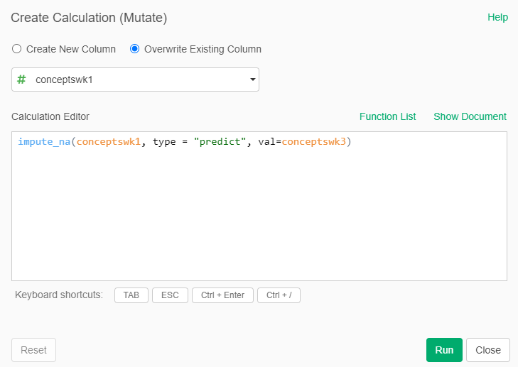
- In the Summary view of the dataset, select the actions that are possible with the column conceptswk1.
- Select “Work with NA” and then select “Fill NA with” and then select “Predict”
- We will predict conceptswk1 based on the values of conceptswk3, given that scores of the students in week 1 should be related to those in week 3. Then the formula should be:
impute_na(conceptswk1, type = "predict", val= conceptswk3)
- Repeat this procedure for the other columns that have missing values, selecting an appropriate variable for the prediction
Scale the Data
First, we scale the data. This puts each variable on a comparable scale with a mean of zero and a standard distribution of one based on its distribution. So for the scaled data, whether a particular value is positive or negative just tells us if it is above or below the mean, and its value tells us how much (in standard deviation units) it is above or below the mean.
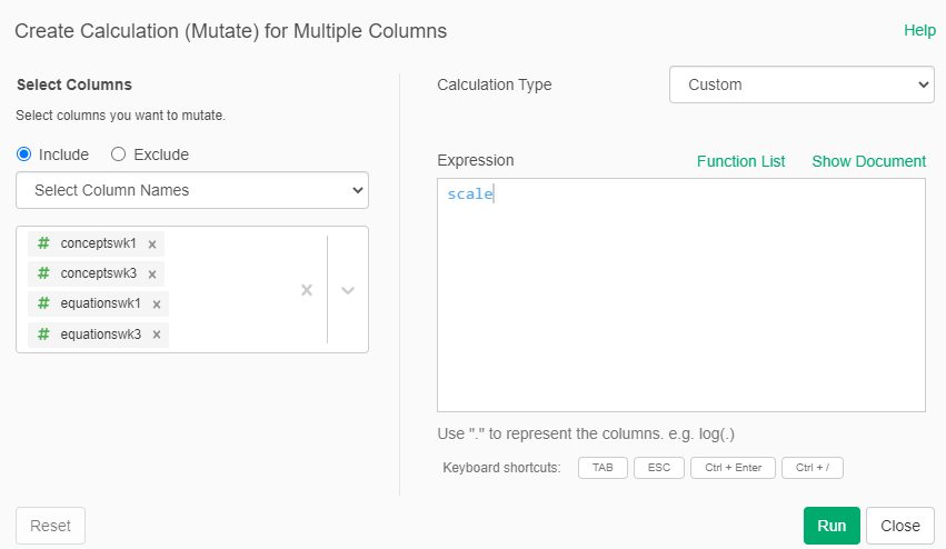
- Add a new Step for the dataset and select “Mutate (Create Calculation) for Multiple Columns”
- Select the numerical columns “conceptswk1, conceptswk3, equationswk1 and equationswk3”
- In calculation type, select “Custom”. In the formula write:
scale
We now notice, that the type of the variables have changed to "array". We need to convert them back to numeric
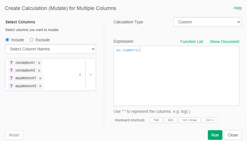
- Add again an new Step for the dataset and select “Mutate (Create Calculation) for Multiple Columns”
- Select again the same columns
- In the calculation type, again select “Custom” and in the formula write:
as.numeric
Now the variables should be centered around 0 with a standard deviation of 1
Decide How Many Clusters to Look For
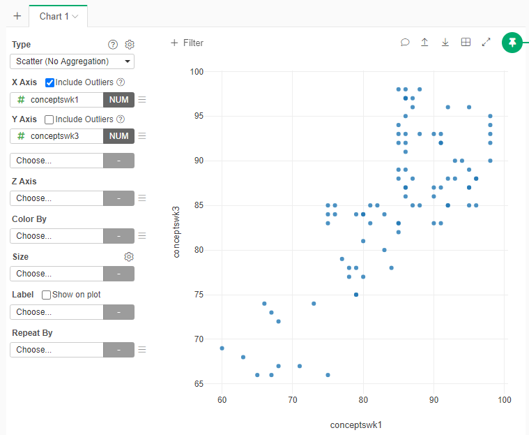
Now let's look at how the different observations are similar / different across the different variables to assess what k (# of clusters) we might be looking for. We will create four different scatter plots * Add a new Scatterplot Chart * Select as variables X=conceptswk1, Y=conceptswk3
- Create additional Scatterplot Charts for the following pair of variables
- X=equationswk1, Y=equationswk3
- X=conceptswk1, Y=equationswk1
- X=conceptswk3, Y=equationswk3
Based on the Scatterplots how many clusters of students do you think there might be? Explain why
- One interpretation: Based on the “Conceptswk1/Conceptswk3” scatterplots, I think there are 3 clusters of students. They are a) students who get high scores; b) students who get medium scores ; c) students who get low scores; on the concept sections of both quizzes. Based on the “Equationskw1/Equationswk3” scatterplots, I think there are 4 clusters of students. They are a) students who receive high scores on the equation sections of both quizzes; b) students who receive medium scores on the equation sections of both quizzes; c) students who recieve low scores on the equation sections of both quizzes; d) students who make an improvement in the equation section in week 3’s quizzes comparing to week 1’s. Therefore, I think there are 4 clustering in total. They are a) students who always get good score; b) students who always get medium score; c) students who always get low scores; and d) students who make an improvement in the equation section of week 3’s quizzes.
Cluster the data
- Add a new Step -> Run Analytics -> K-Means Clustering
- Include the columns “conceptswk1, conceptswk2, equationswk1, equationswk3”
- Select the number of clusters that you think should be in the data

- Run the Analysis and see the new cluster variable
Visualize the clusters
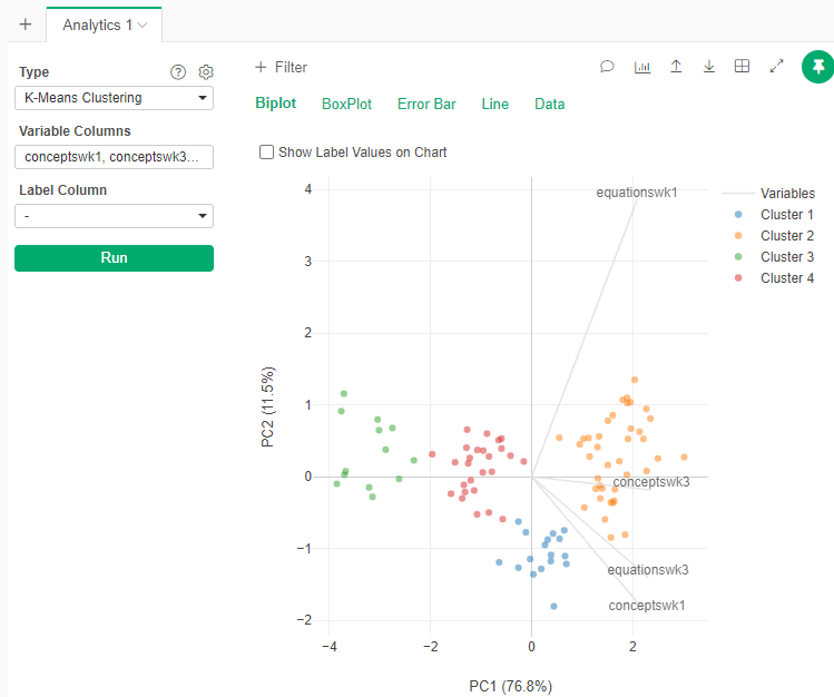
To get a visual representation of the clustering, we will use the Analytics tab
- Go to the Analytics tab
- Select Type: K-Means Clustering
- Select the same variables
- In the gear beside Type, select the number of clusters that you think the data has
- Run the Analytics
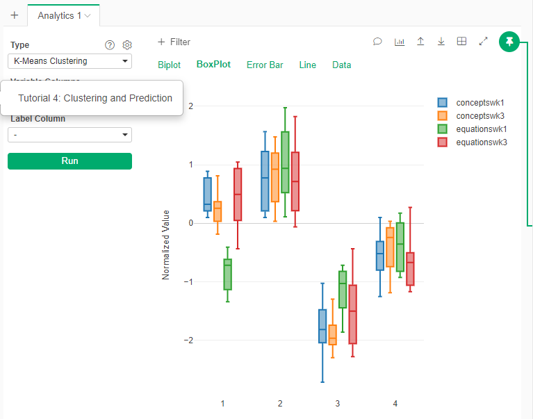
- Check in the other visualizations (BoxPlot)
- Another way of visualizing the clusters is to repeat the scatterplots between variables but using the cluster information to color the points:
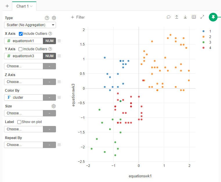
Does the number of clusters that you selected seems to be clear separations of data in the plot? Why?
- One interpretation: The 4 clusters seem to have clear separations of data in the plot, which means the assumption of 4 clusters is correct. Furthermore, by checking the detailed information of the blue points in each scatterplot, I found that the differences between “Equationswk1” and “Equationswk3” are larger than the differences between “Conceptswk1” and “Conceptwk3”, which means students have greater improvement in chemistry equations than in concepts. There are several reasons that could lead to this condition: a) equations are harder to learn than concepts; b) most students come with a better understanding of concepts; c) some students were able to make for their lack of understanding of equations by the instructor classes during those 2 weeks.
Check the number of clusters
We will analytically check the number of clustes
- Add a new Analytic
- Select K-Means Clustering
- Select the same variables to include
- In the options of the Analysis (Gear just beside the type of the Analytics and the Help), in the section “Elbow Method” select “TRUE”
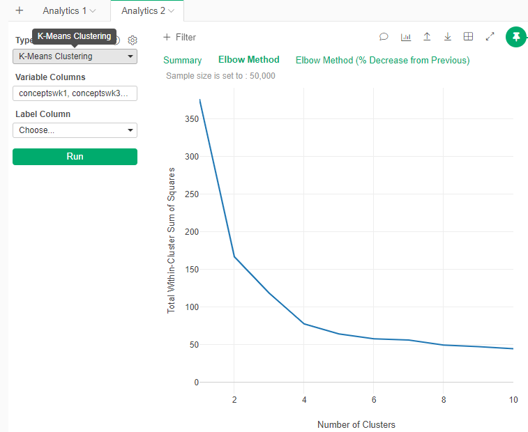
Observe the resulting graph
- This graph is how much information each new cluster add. Usually you want to cut at the “Elbow”, or the point where the gain in information start to decrese.
What is the ideal number of clusters according to the “Elbow” graph?
- It seems to be between 3 and 4. It seems to be in line what we originally selected.
Clustering Discussion
Based on all the analyses above:
What, if any, ethical issues are there related to the application of this analysis to inform instruction?
- One opinion: An ethical issue that I could think about is that the instructor will assign stereotypes to the students, especially students with bad performance in both quizzes. The instructor may be conviced by the clustering that some students just cannot make improvement, so that they will not try to help these students. It is also harmful for instructors to believe that good students will always do good job whether they receive assisstance from the instructor or not.
Do you think clustering was a useful approach in this situation? Why or why not?
- One opinion: I think clustering is a useful approach in this situation, because it allows the instructor to establish a preliminary understanding of the student and the class. It helps the instructor to know who are the student that need more support. It could also be used as an indicator of the effectiveness of the pedagogy.
Reporting
Now you need to create a Note report where you will explain your findings to the instructor. Use as many graphs and explanations as you see fit.