Tutorial Four: Visualizations
Loading Data
For this tutorial we will use a dataset ofered by the Integrated Postsecundary Education Data System (IPEDS). It contains information about colleges and universities in the US.
For each institution, it has a lot of information. For example: number of students registered, higher degree offered, number of international students, geographical location, number of graduates. For more information, please visit: https://nces.ed.gov/training/datauser/IPEDS_01.html
We obtained a short version of the data from a Kaggle Project (https://www.kaggle.com/sumithbhongale/american-university-data-ipeds-dataset/version/1)
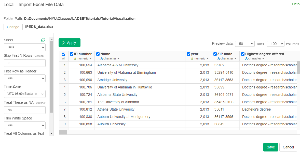
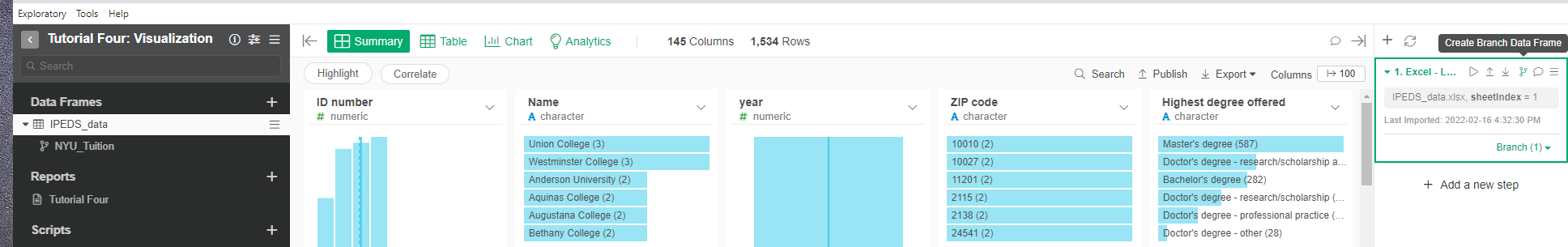
Import the Excel file "IPEDS_data.xlsx". Name the dataset "IPEDS_data".
Visualizations
Bar Charts with just one type of value
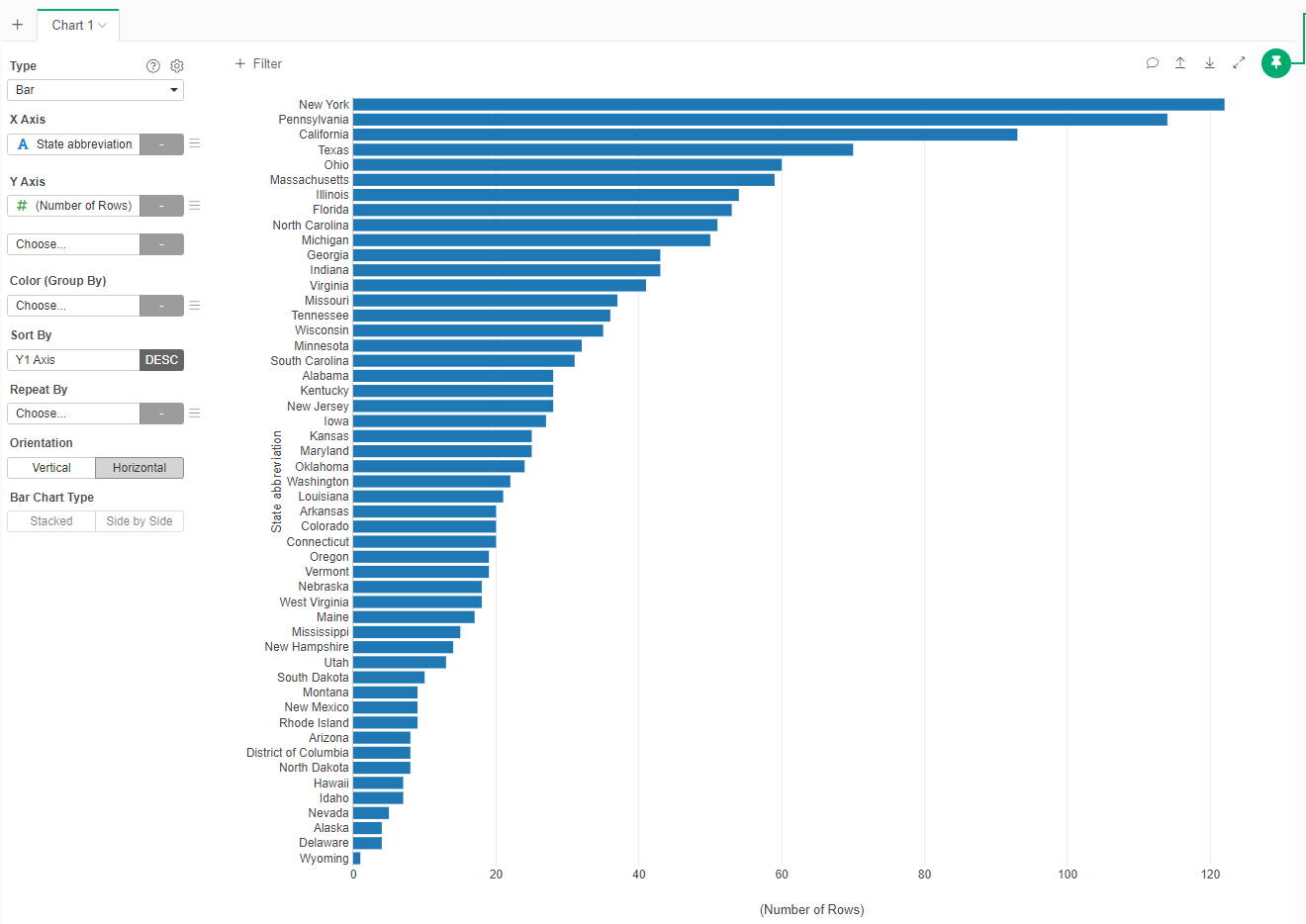
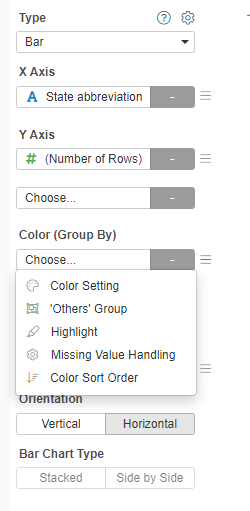
First we will create a bar chart with the number of Universities per State. For this we will show show how many of institution (each institution is a row) belong to each state. For this:
- Go to charts, add a new one.
- Select "Bar"
- In X Axis search for "State abbreviation
- In Y Axis search for # (Number of Rows)
- Sort By "Y1 Axis"
- Orientation "Horizontal"
- Maximize to see all the names.
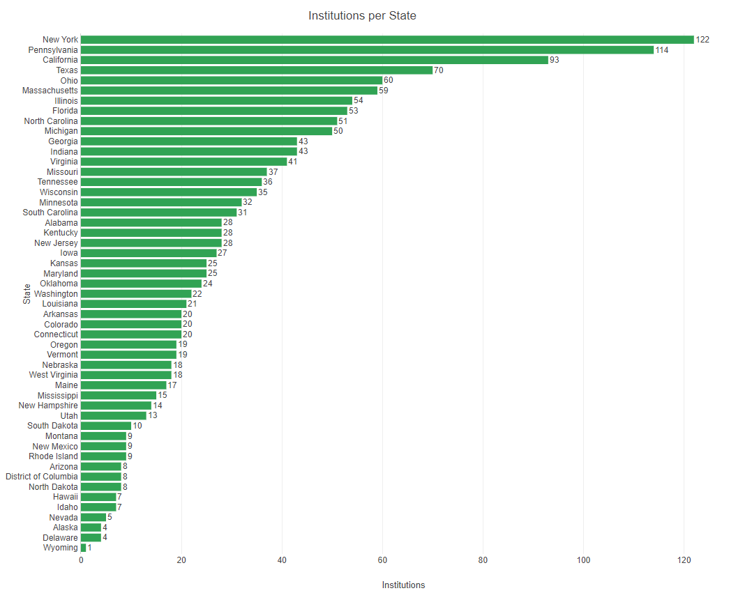
While the visualization is correct, we would want to improve its apperance. We would want to add a title, axis labels and show the value on each bar.
Click on the gear beside the Type option
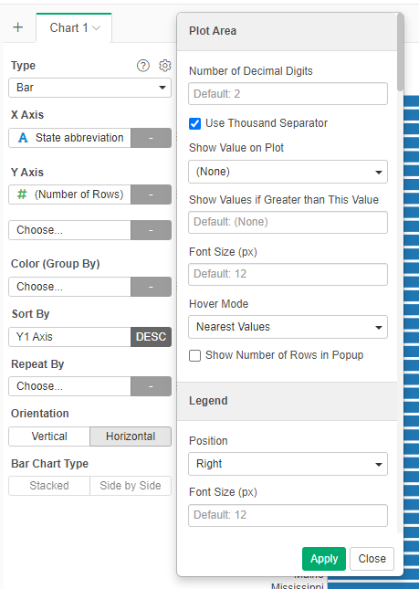
- In the Title section, set Text to "Institutions per State"
- In the X Axis Title section, set Title Text to "State"
- in the Y Axis Title section, set Title Text to "Institutions"
- in the Plot Area section, set Show Value on Plot to "Above"
Apply and close
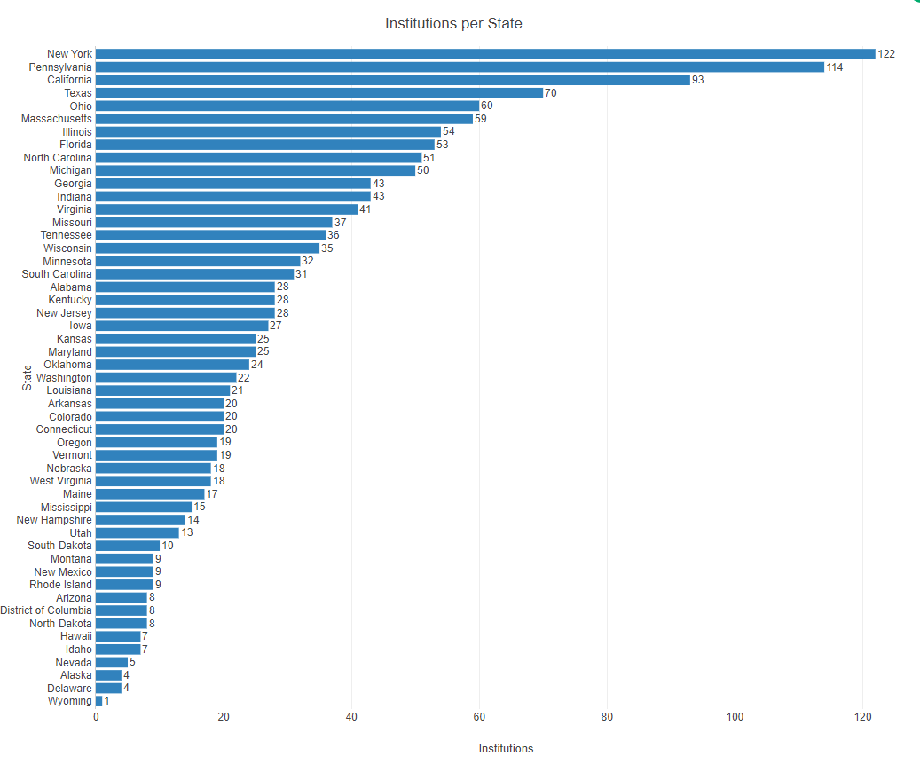
Now lets change color.
- Click the three line menu besides Color (Group By)
- Select Color Setting
- Select any Color Palette (only the first color will be used as there is only one type of values)
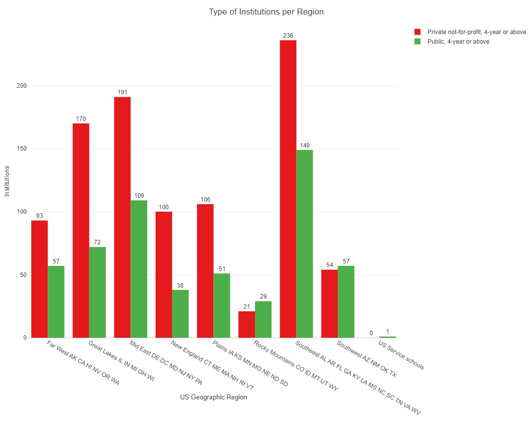
Bar Graph with categories
We will now create a chart that presents the sector of the institutions (Private or Public) per Geographical Region.
- Create a new Chart, select Type Bar
- In the X Axis, select "Geographic Region"
- in the Y Axis, select "# (Number of Rows)"
- In the Color (Group By), select "Sector of Institution"
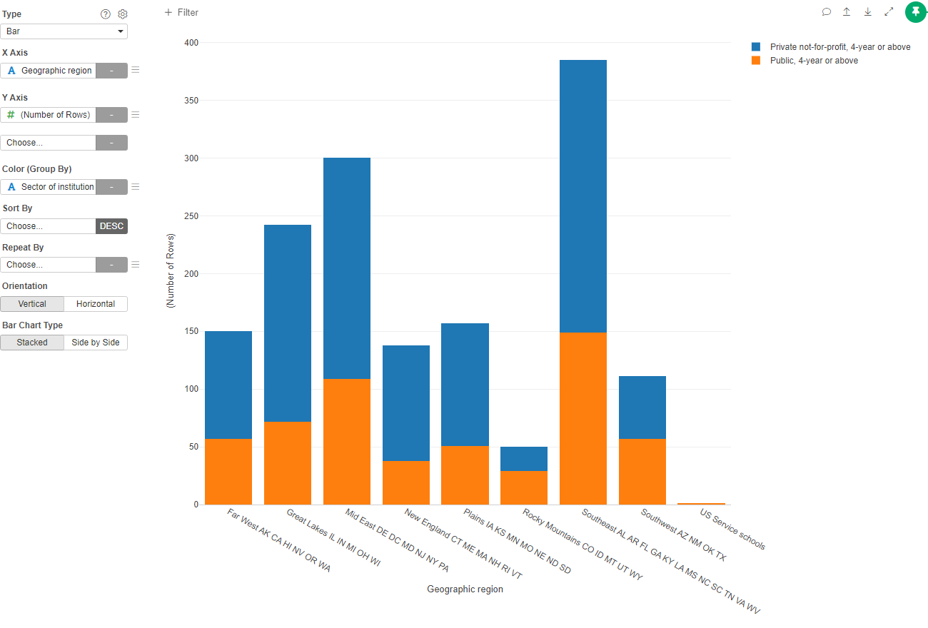
By default, Exploratory create a Stacked Bar Chart. If we want to have the different sectors side by side:
- Click on Side by Side in the Bar Chart Type
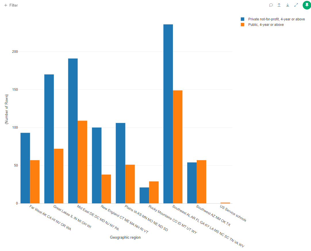
Now, on your own, add a Title, labes for the X and Y axis, show values for the columns and change the color Palette.
Line Chart with a single category
We now would want to see how the tuition values have increased in New York University. To do this we will create a copy of the data to do some filtering and wrangling.
- First go to the Step section and click on the "Create Branch Data Frame" icon.
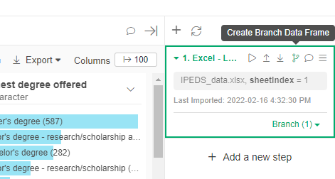
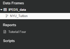
- Call the new dataset "NYU_Tuition"
- Now click on "NYU_Tuition" in the Data Frames Section
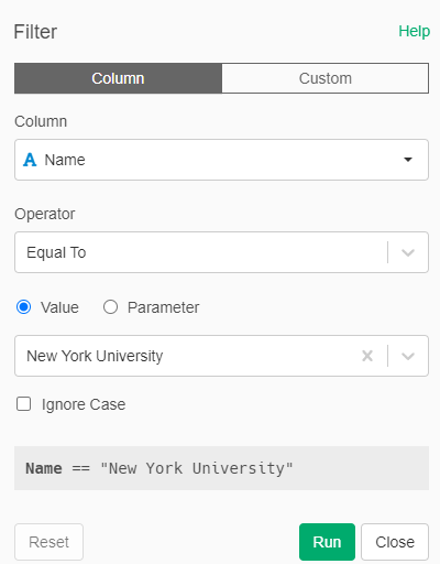
- Add a new step: Filter
- Filter by the "Name" of the Institution. In operator select "Equal To". In values select only "New York University"
- Run the Filter
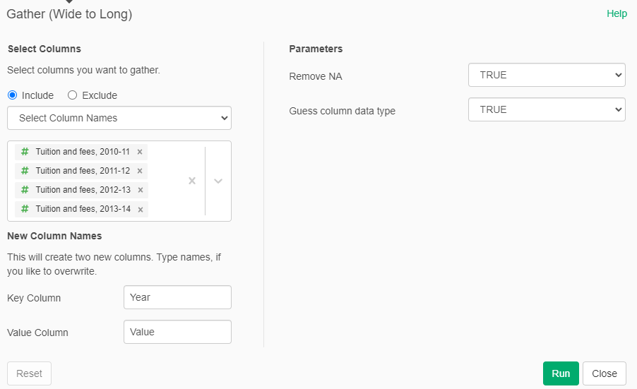
Beacuse the different tutions in 2010, 2011, 2012 and 2013 are different columns, we need to gather them into a single column. To do this we convert from wide to long.
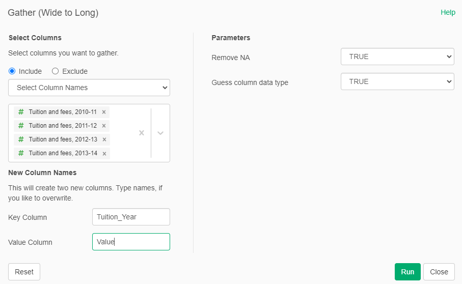
- Add a new Step: Gather (Wide to Long)
- Inlcude all the "Tuition and fees: 20XX - XX" columns
- The Key column will be called "Tuition_Year"
- The Value column will be called "Value"
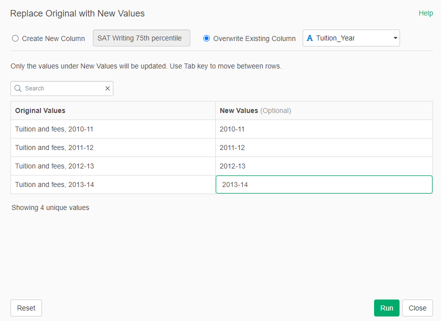
Now we will change the value in the "Tuition-Year" column to remove inneceary text.
- Go to any column in Summary and click on its triangle and select "Replace Values -> "With New Values"
- In the options, Select Overwrite Existing Columns and select "Tuition_Year". The values of the column should appear as in the image below.
- Set the values to only the years
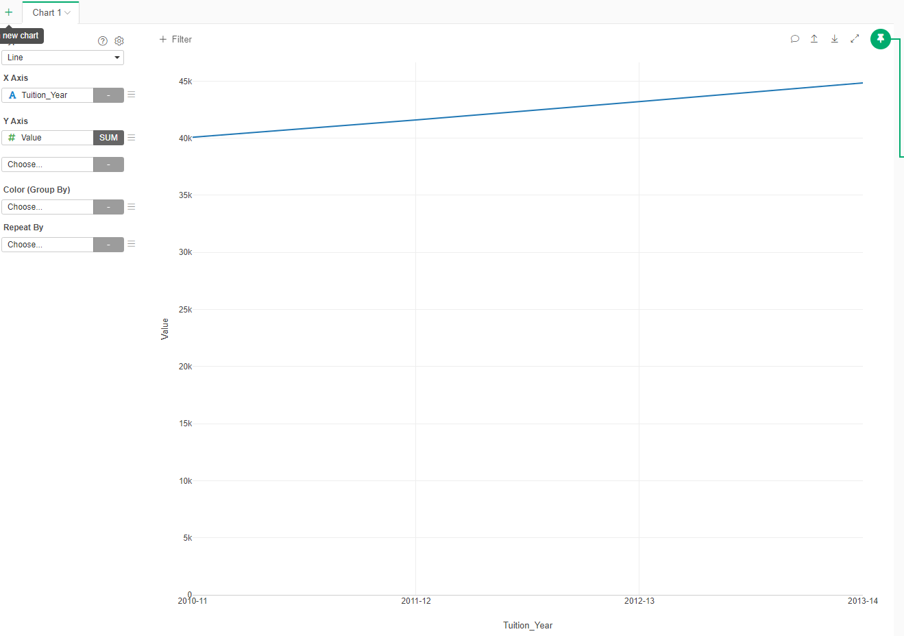
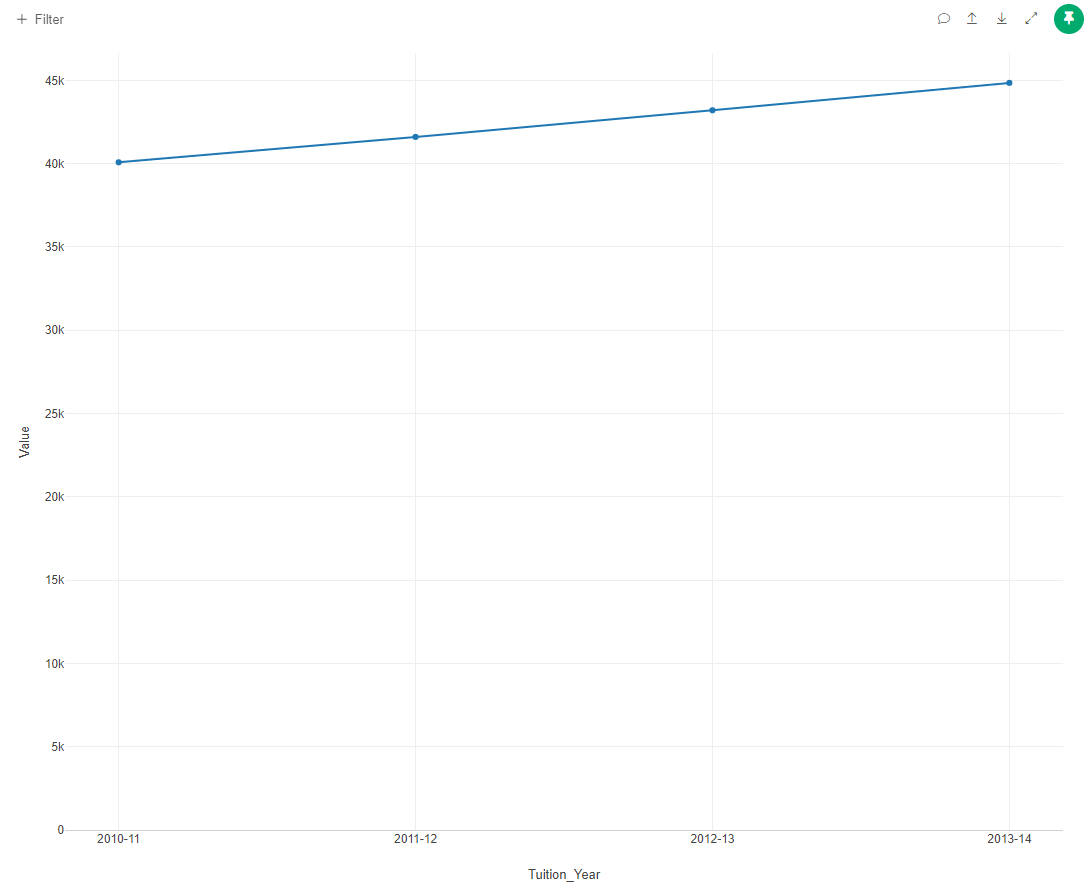
Now we have the data in the format that we needed for creating our chart:
- Add a new Chart
- In Type select "Line"
- In the X Axis select "Tuition_Year"
- In the Y Axis select "Value"
To make the graph a little more readable, lets add points in the line:
- Click on the three line menu beside the Y Axis
- Select Marker
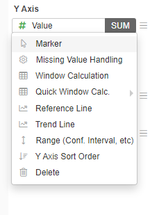
- In Marker, select "Line + Circle"
- Apply
Add title, labels and colors to finish the chart.
Line with several categories
Now we will chart how the the tuiton has changed in different regions.
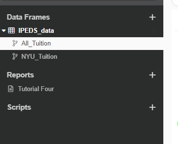
- Return to the IPEDS_data and create a new branch called "All_Tuition"
- Click on the new "All_Tuition" dataset
- Create a new step: Gather (Wide to Long) select the Tuition columns. The key column will be called "Tution_Year" and the value column will be called "Value"
Now we will summarize according to the geographical region
- Add a new Step: Summarize (Aggregate)
- Group By "Geographic region" and "Tuition_Year"
- The Value will be "Value"
- The aggreation fuction will be "Mean"
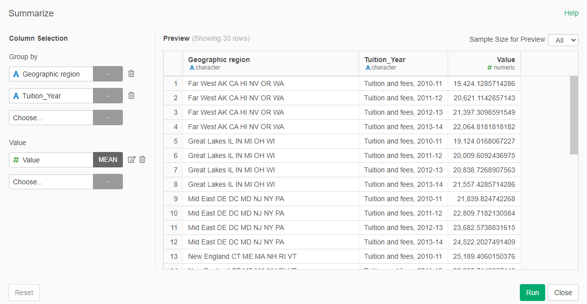
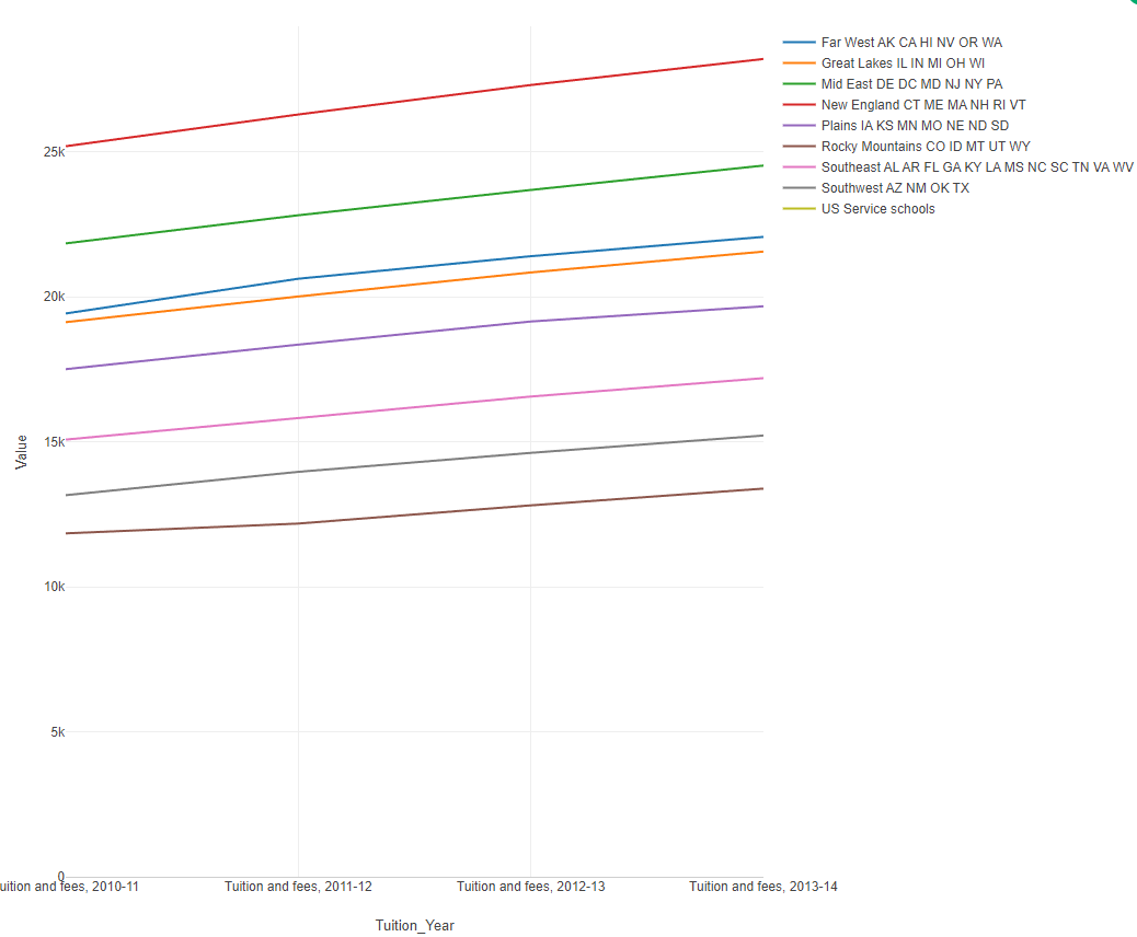
With the dataset ready, we proceed to create the graph
- Add a new Chart, select Line
- In the X Axis select "Tuition_Year"
- In the Y Axis select "Value"
- in Color (Group By), select "Geographic region"
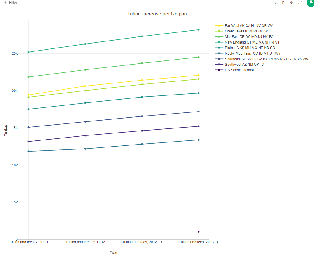
Now that you know how, improve the chart adding a circle ot the line to make it more legible, add a title, labels and select another color palette.
Pie Chart for yes o no
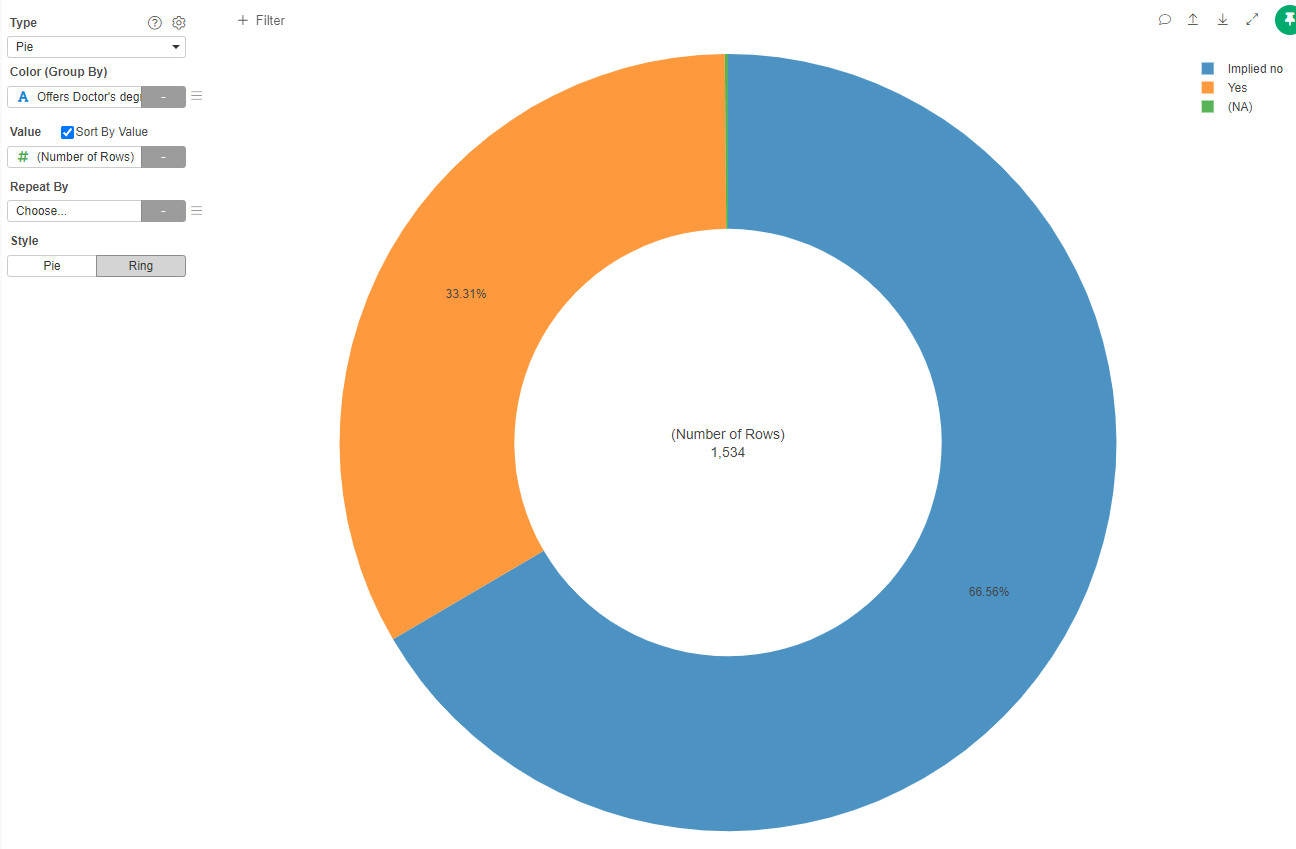
Now we will see how many of the institutions offer research doctoral degrees.
- Retun to the original IPEDS_data
- Create a new chart Type Pie
- For Color, select "Offers Doctor's degree - research/scholarship"
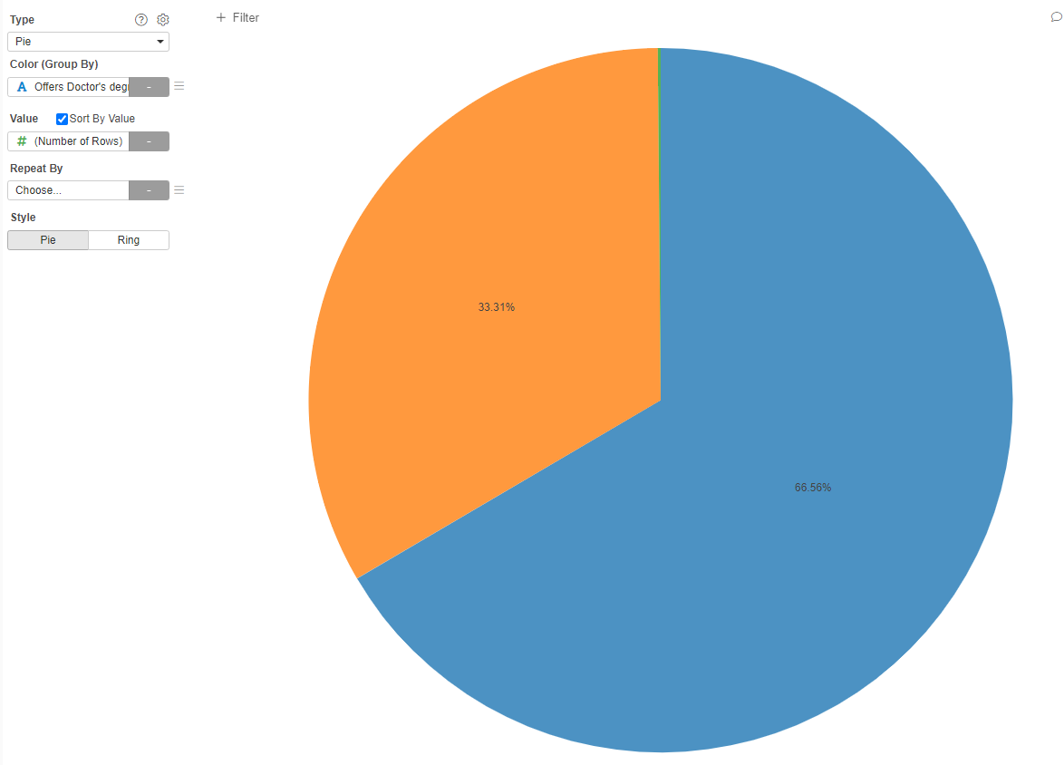
Now, you can select between Pie or Ring (purely asthetic):
If we would want to see the percentages per Geographic region:
- In Repeat By select "Geographic region"
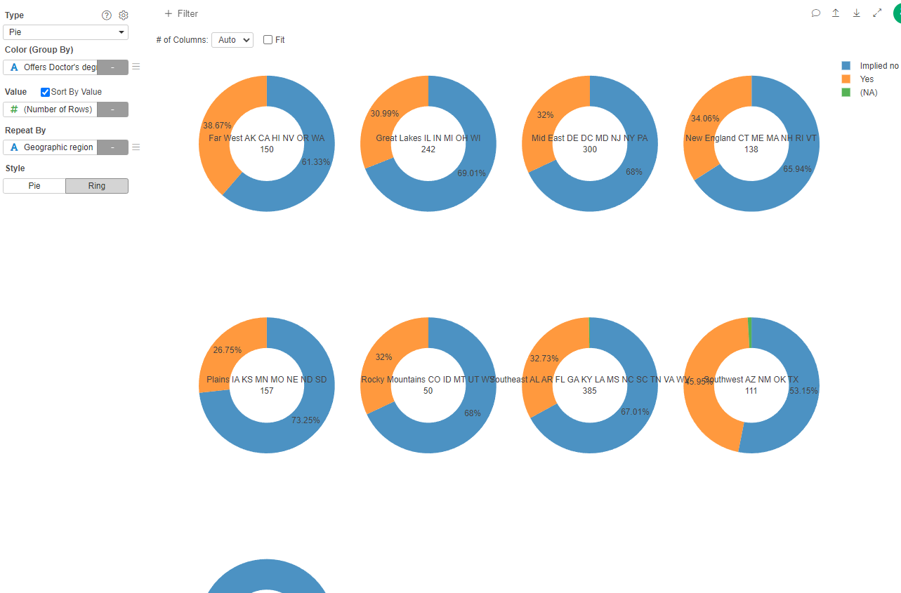
You can experiment with the colors and other settings that you already know.
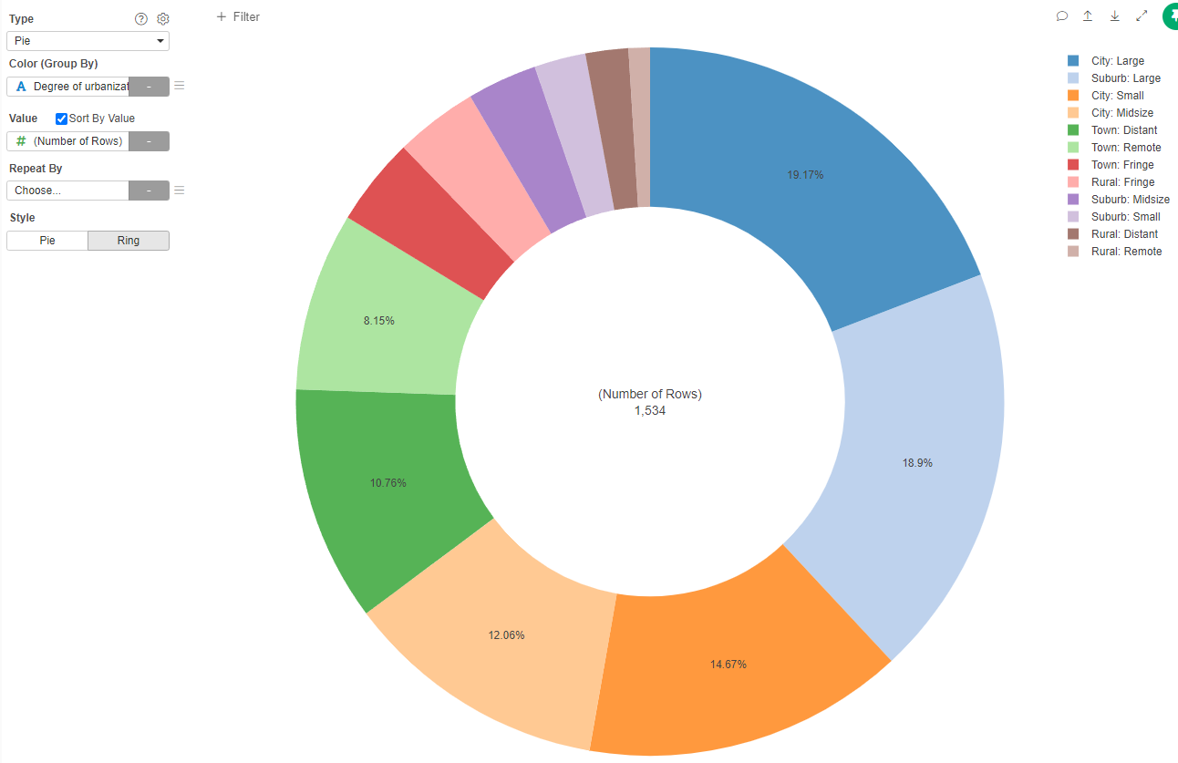
Pie chart with several values
Now we will see in which urban or rural environment these institutions are located.
- Create a new Chart, type Pie
- In Color select "Degree of urbanization"
- in Value select "# (Number of Rows)"
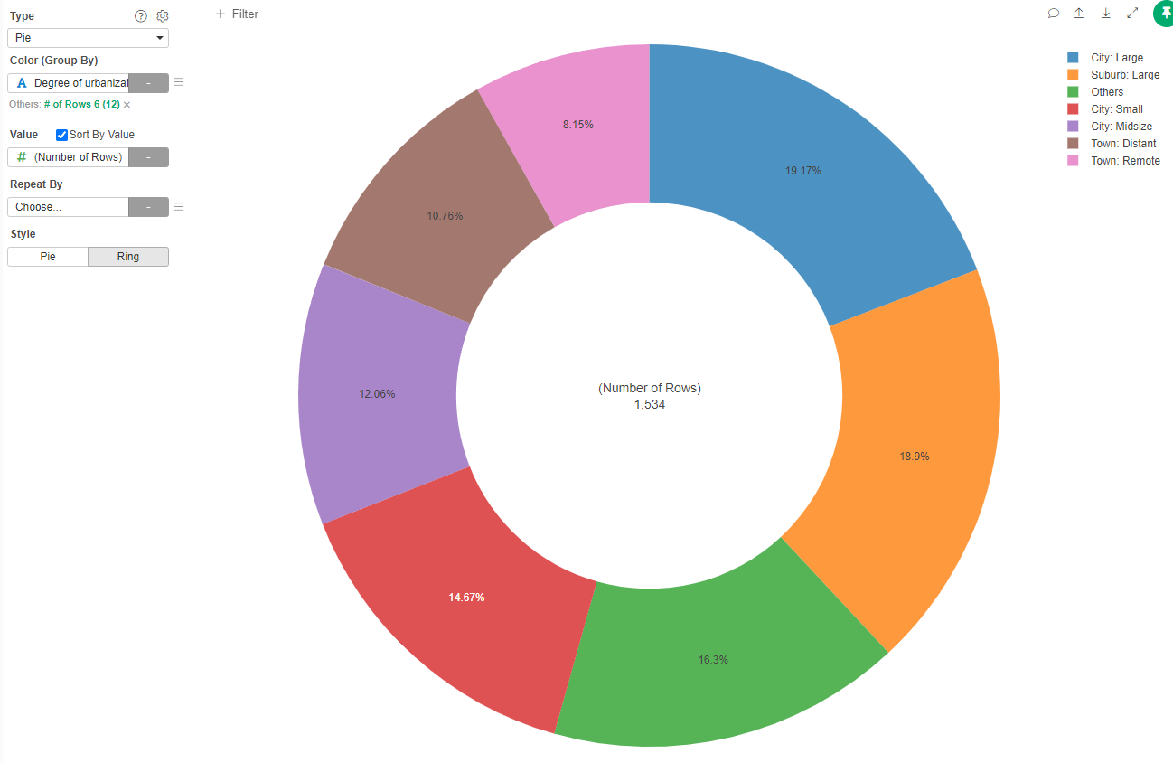
Because there are some categories that are unfrequent, we can create a category "Other" to group them.
- Click on the three line menu in the Color (Group By)
- Select the "Others Group"
- In Type select "Based on Number of Rows"
- In Keep Top N Frequent, type "6" (The six more frequent)
- Apply
Boxplots
Imagine that we want to know the distribution of the size of the institutions (number of students enrolled) according if they are public or private universities.
- Create a new Chart, type Boxplot
- in X Axis select "Sector of the Institution"
- In Y Axis select "Enrolled Total"
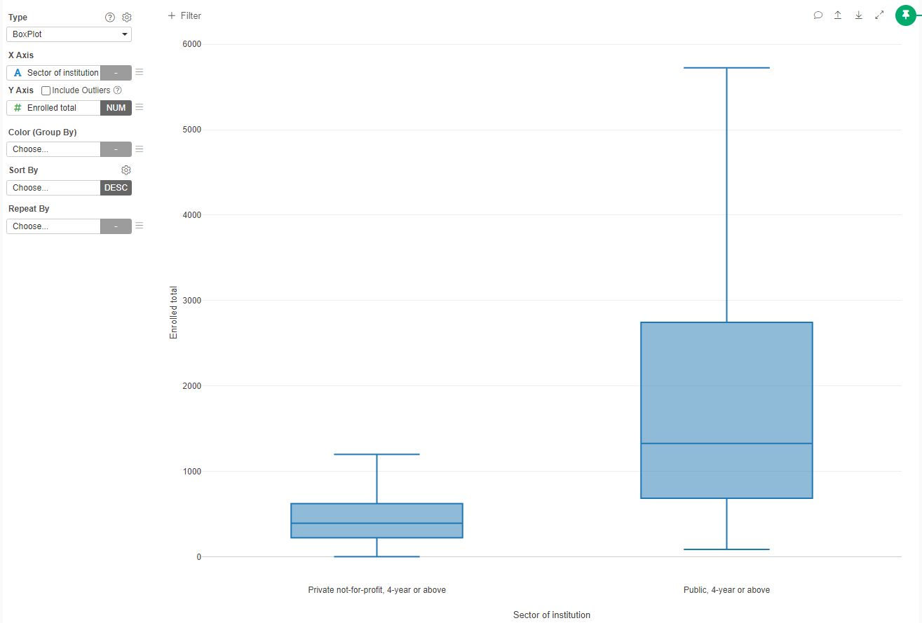
We can see that public Universities tend to have more students that private universities. Does this trend is the same depending on the maximum degree they provide? To answer this question, we need to first convert "Highest degree offered" into a factor an order it in increasing level of degree.
- Convert the "Highest degree offered" column to Factor
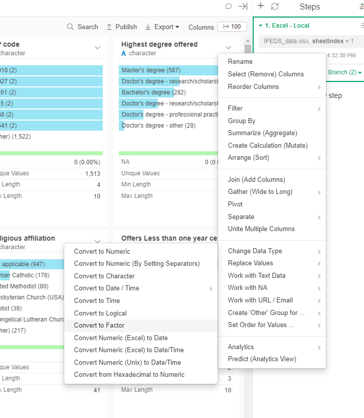
- Manually reorder the factor
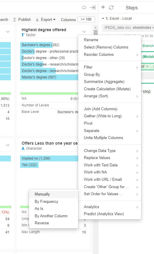
The order should be:
fct_relevel(`Highest degree offered`, "Bachelor's degree","Master's degree","Doctor's degree - other","Doctor's degree - professional practice","Doctor's degree - research/scholarship and professional practice","Doctor's degree - research/scholarship")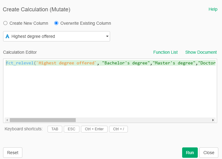
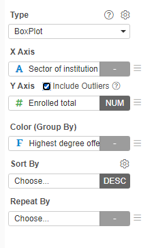
- Now create a new chart type Boxplot
- In X Axis set "Sector of Institution"
- In Y Axis set "Enrolled total"
- In Color (Group By) set "Highest degree offered"
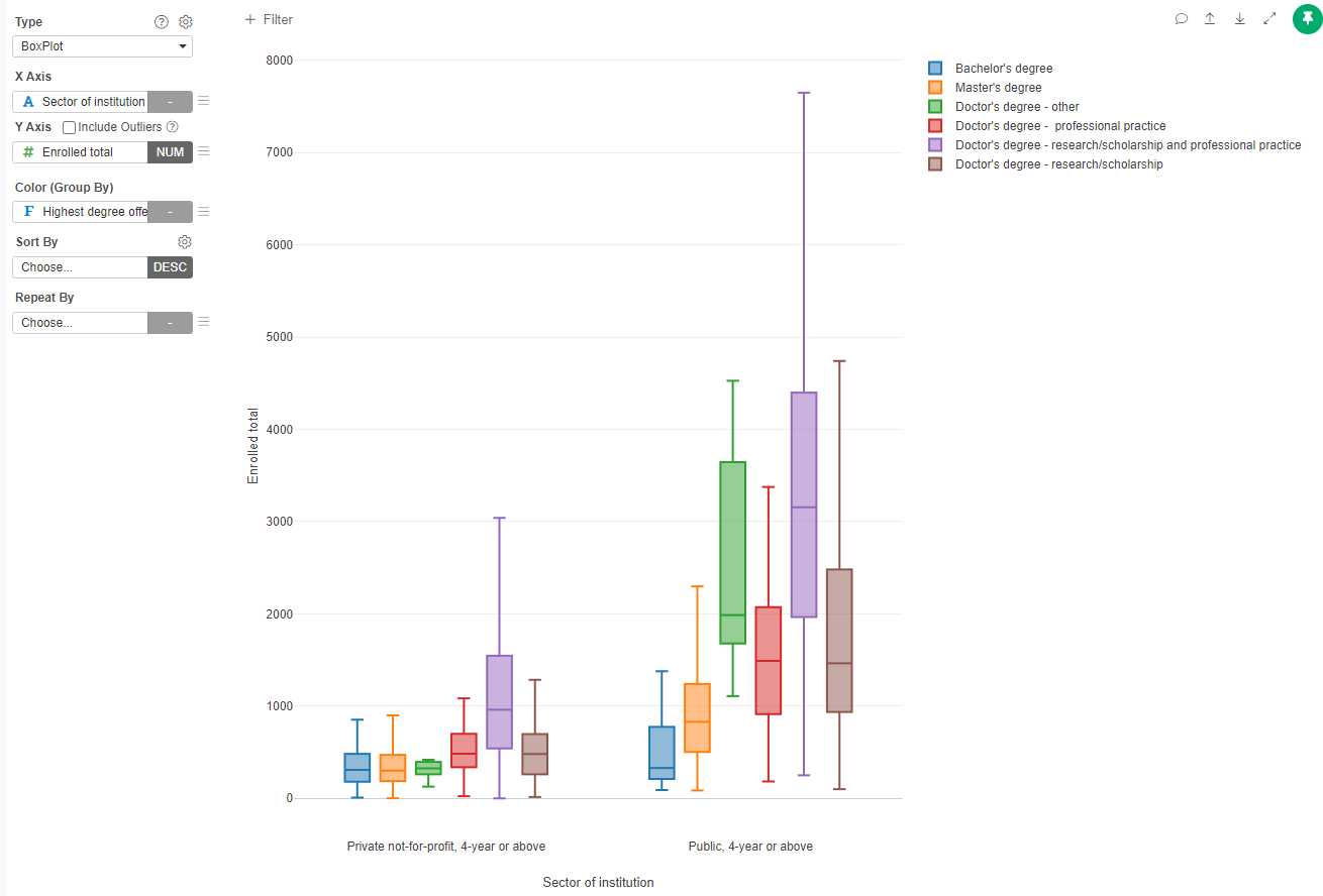
You can decide if include or exlude outliers (those that are beyond the 1.5 Interquartile Range - IQR)
Plays with colors and add the title and labels to the graph.
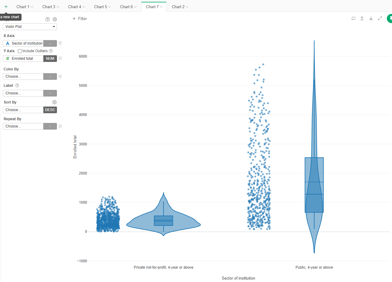
Violin Plots
This are another version of the boxplots. Let's recreate the previous chart.
- Create a new chart, type Violin
- X Axis: Sector of Institution, Y Axis: Enrolled total
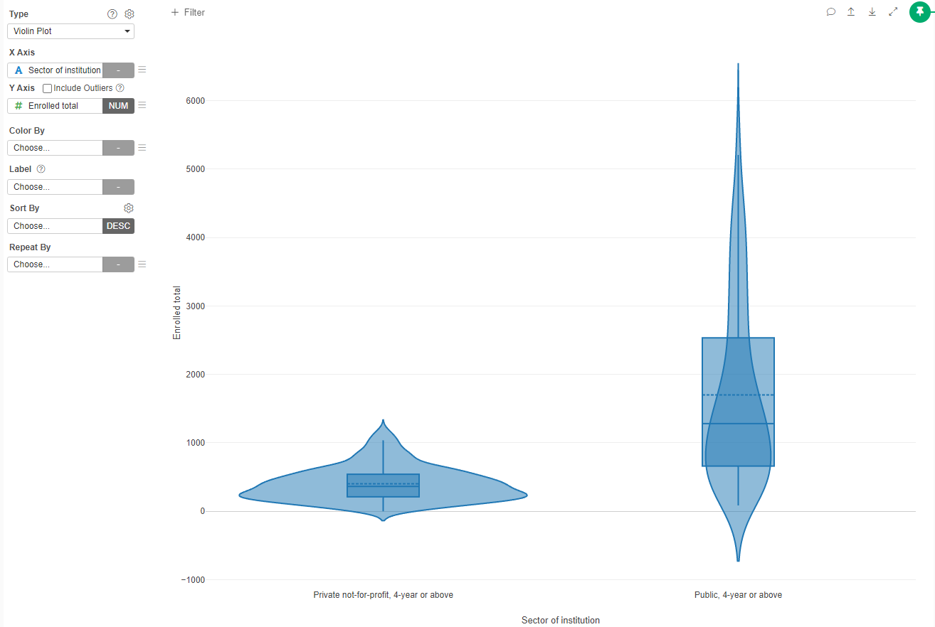
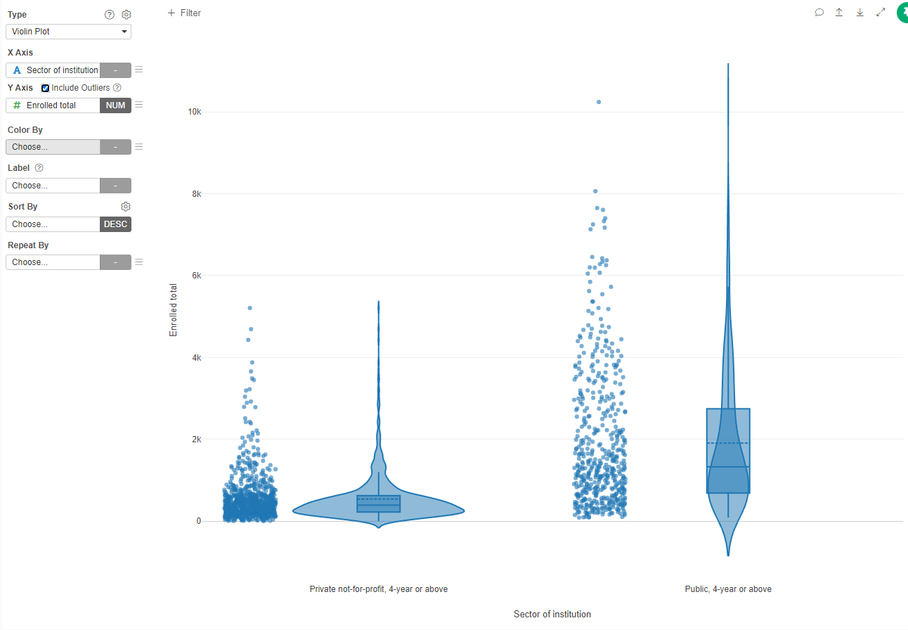
We can see that additionally to the boxplot, we can see the density distribution of the values. To make it clearer we can add the datapoints.
- Click on the gear beside the Type of plot
- Click on "Show Data as Points"
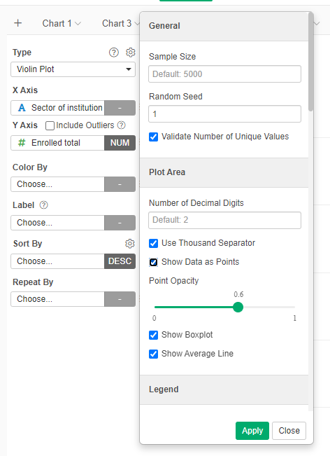
- Apply
- Select "Include Outliers"
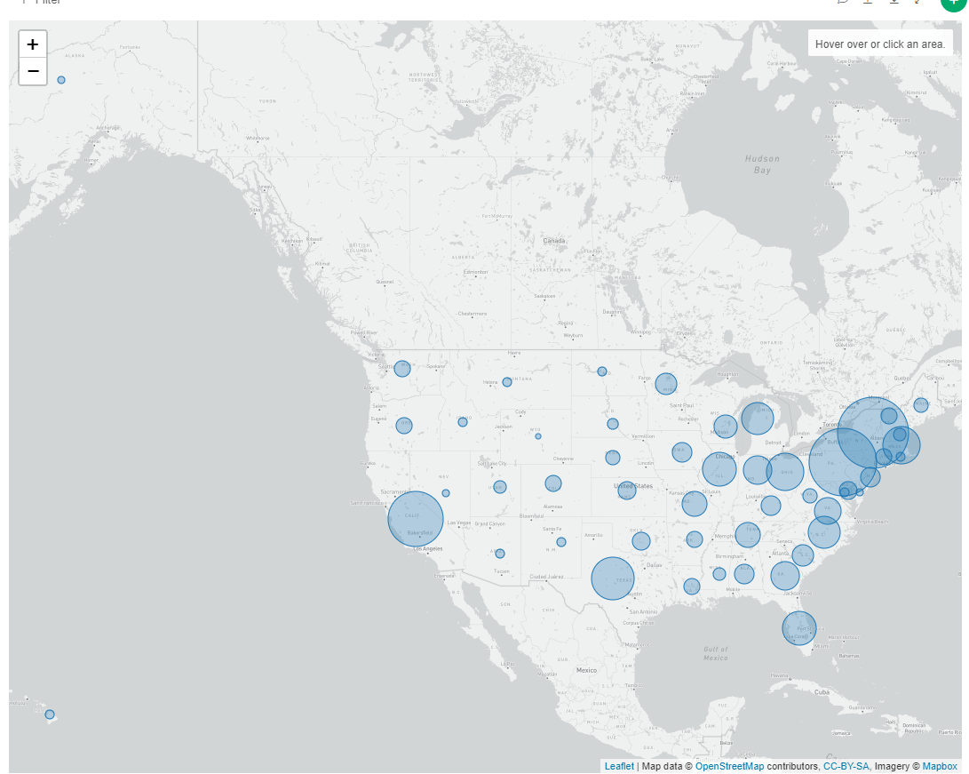
Map aggregated by state
Given that we have the name of the state on which each institution is, we can map aggregates by state in an map. Lets create a map that show the number of institutions per state.
- Create a new Chart type "Map - Standard"
- In Map, select US States
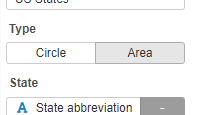
- In State, select State abbreviation
- Size By "(Number of Rows)"
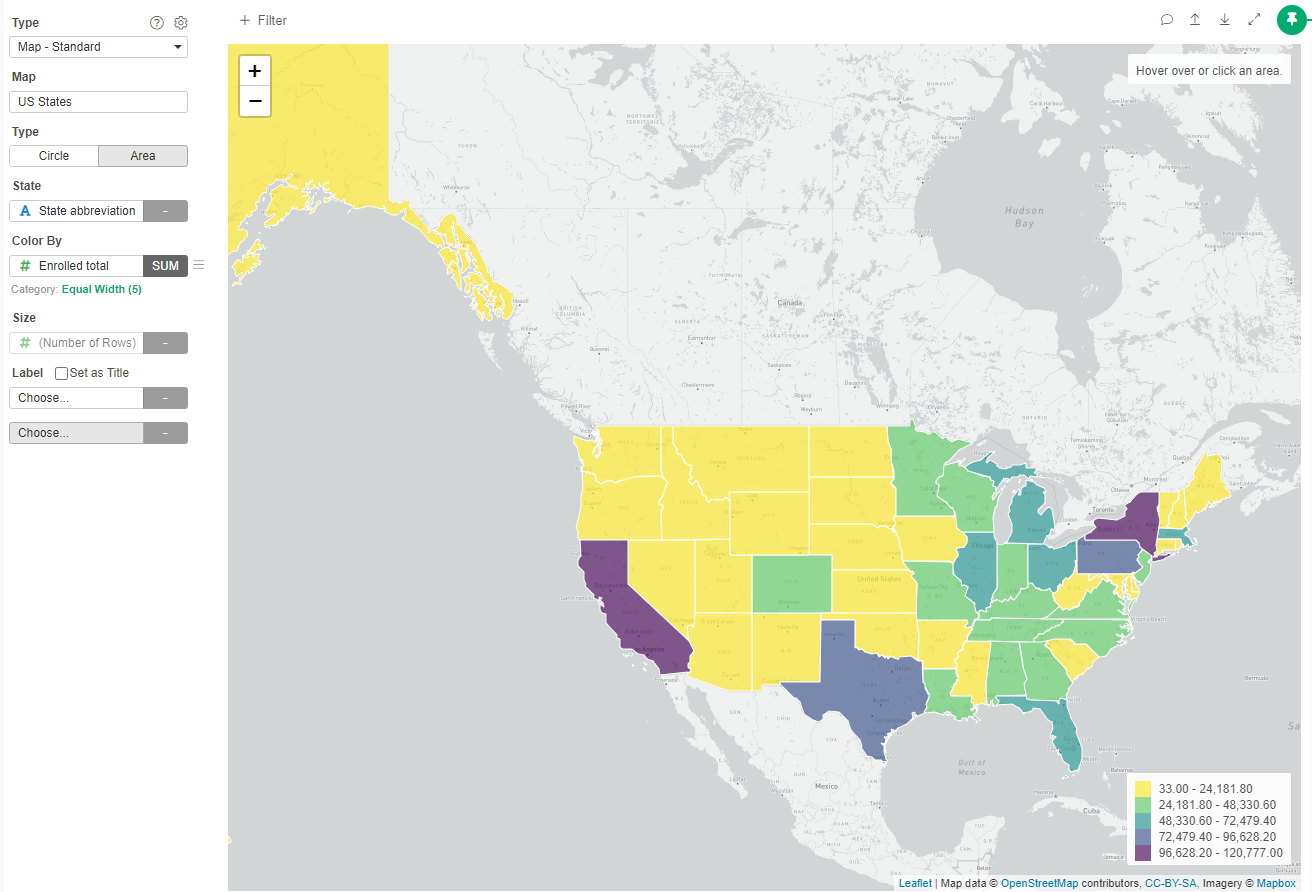
Now we can color them according to any variable, for example, let's color them by the sum of all the students enrolled in that state.
- Color By: Enrolled Total (SUM)
- Choose color pallette "Viridis"
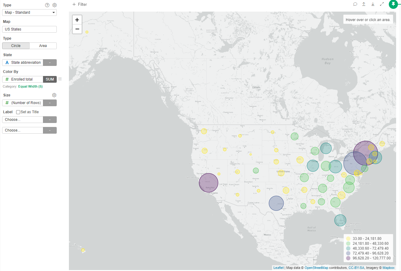
Instead of Circles, we can color each state.
- Select Type Area
Map by zipcode
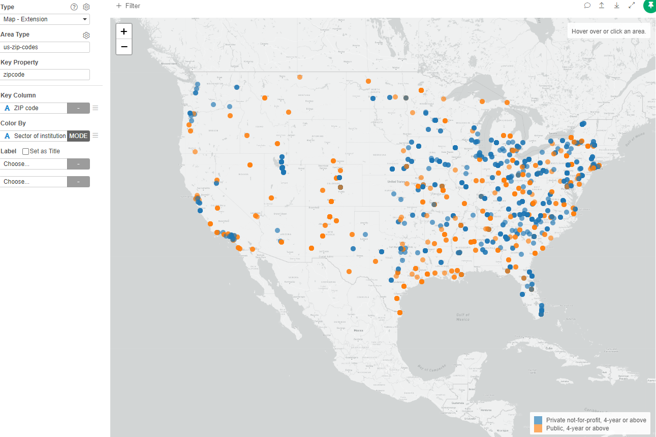
We will now present a map of the institutions colored accordingly to they sector (public or private).
- Create a new Chart, type "Map Extension"
- Area Type: us-zip-codes
- Key property: zipcode
- Key Column: "ZIP code"
- Color By: "Sector of institution"
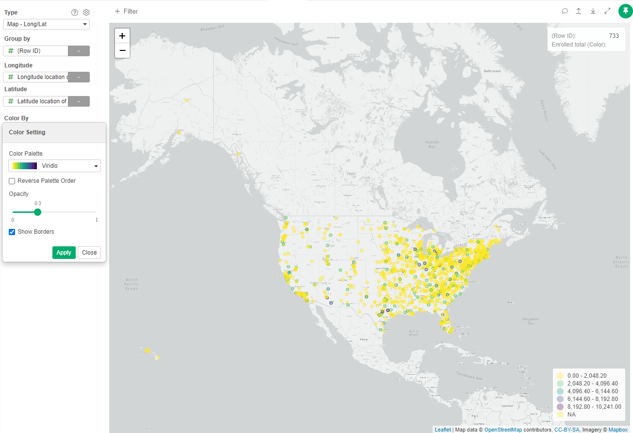
Map by coordinates
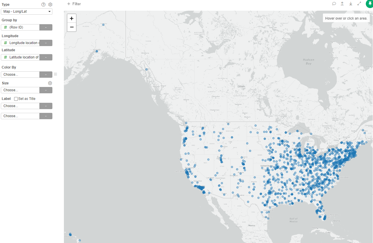
Now we will want to visualize each institution by their geographic coordinates
- Create a new Chart, type Map - Long/Lat
- Group by: "Row ID"
- Longitude: "Longitude location of the institution"
- Latitude: "Latitude location of the institution"
- Select Color By: "Enrolled total"
- Change palette to Viridis
Let's change the type of map and try to find NYU
- Click the Gear near the Type
- In Style Type choose Streets
- In Label, select "Name"
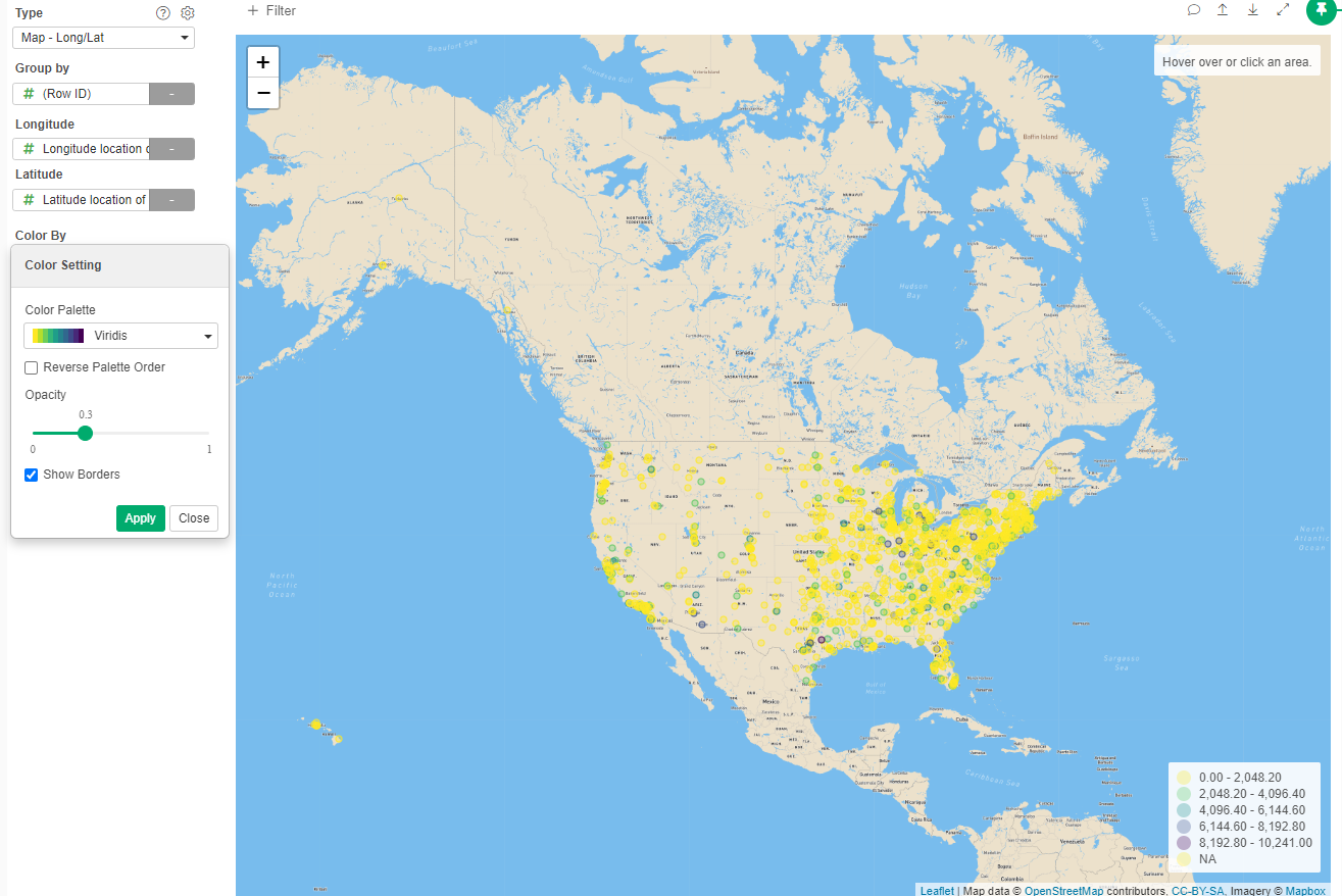
- Zoom to NYC and Washington Square Park
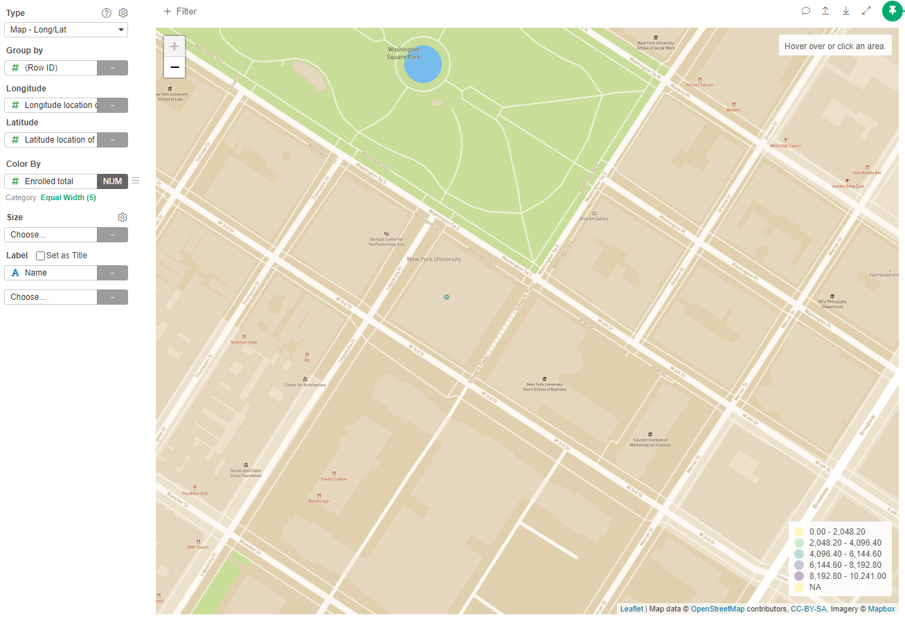
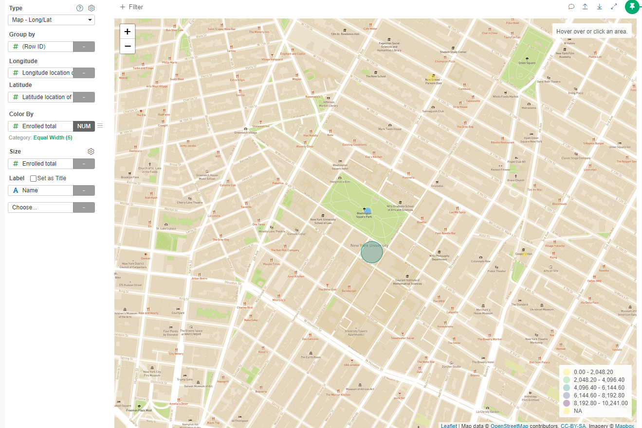
To see it better, change:
- In Size: "Enrolled Total"
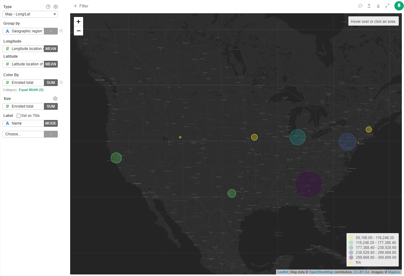
Now, let's group institutions by their geographic region
- Group by: "Geographic region"
- Zoom out
- Change Map Style to Dark
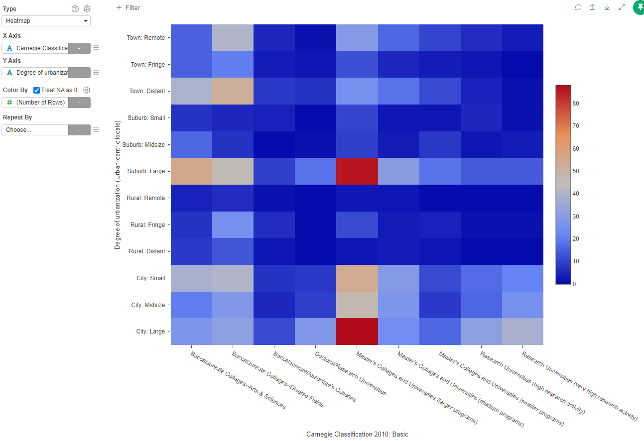
Heatmap
Let's find the most common settings of different types of universities. For this we will use a heatmap:
- Create a new Chart type: Heatmap
- X Axis: Carnegie Classification
- Y Axis: Degree of Urbanization
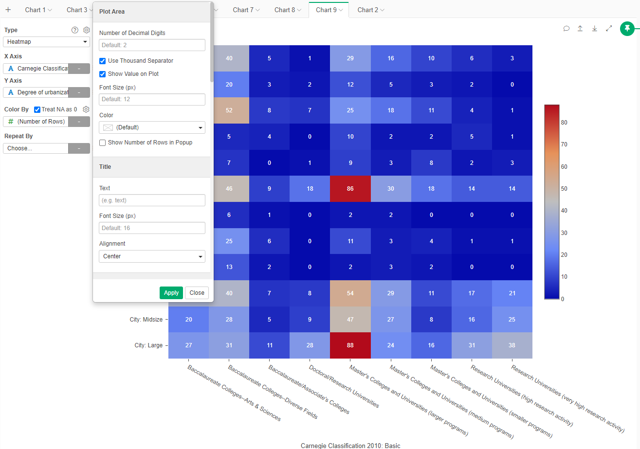
To make it clearer, let's add the value on the plot:
- Click on the gear beside the Type
- Select "Show values in the plot"
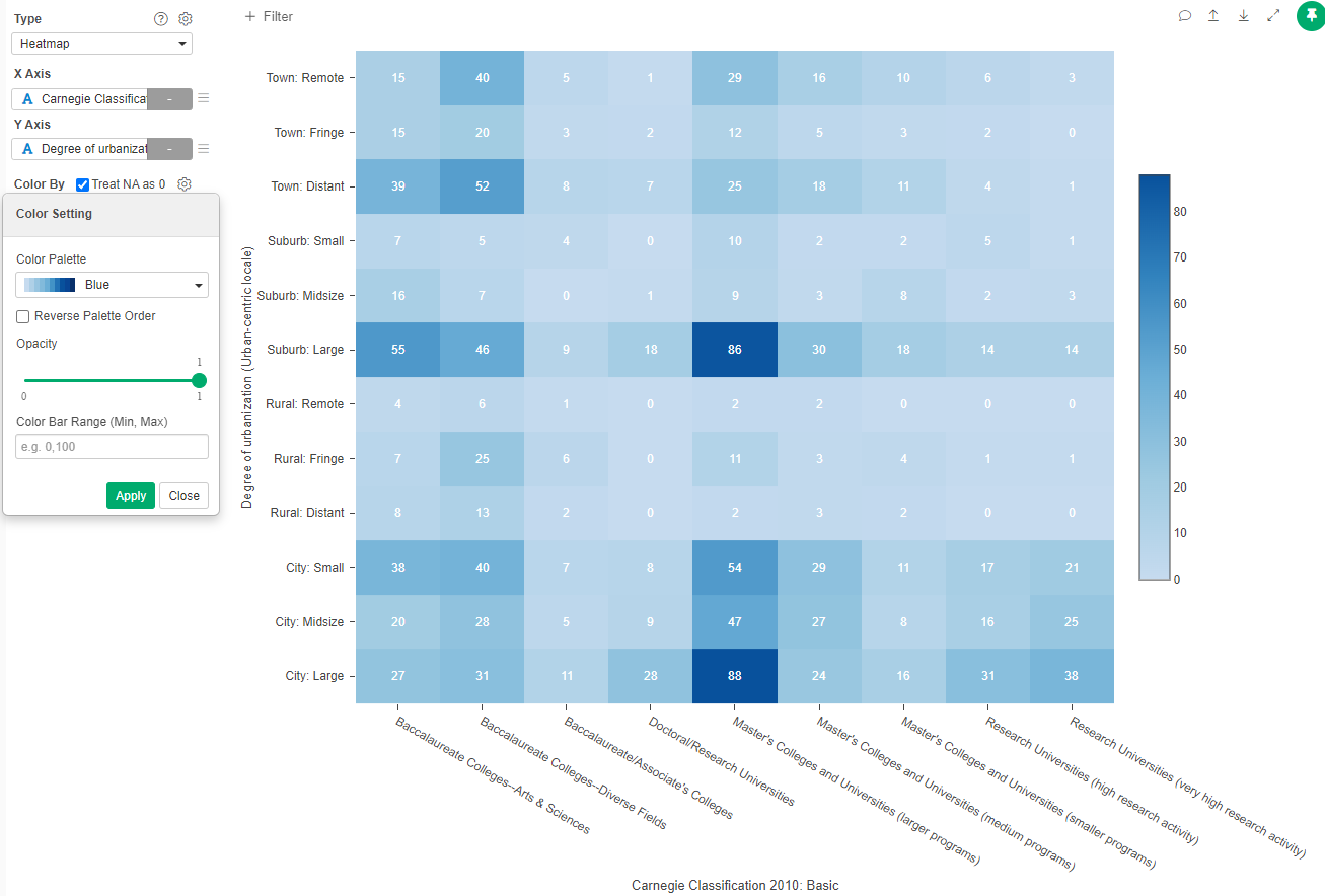
Change the color to make it more salient:
- In the Gear beside Color by, select the Blue (or any other single color) palette.
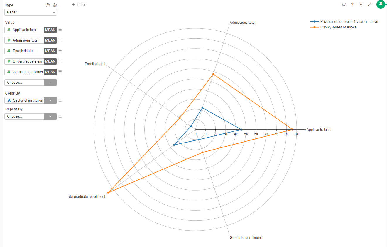
Radar
If we want to compare two individuals or groups based on three to seven dimensions, you can use radar graphs.
- Create a new Chart type Radar
- In values select "Applicants total", "Admissions total", "Enrolled total", "Undergraduate enrollment", "Graduate Enrollment". All of them as "MEAN"
- Color by: "Sector of institution"
Create a Report
Create a note that show all the types of visualizations that you did with a brief explanation of for what do you think they could be useful (the visualization, not the actual data depicted in the chart)
Share that note in Brightspace