Using dplyr to query databases directly instead of using SQL

Let’s say you have airline delay data in your PostgreSQL. To get average departure delay for each state, you can write a SQL query like this.

SELECT "ORIGIN_STATE_ABR", AVG("DEP_DELAY") AS "DEP_DELAY_AVG"
FROM "airline"
GROUP BY "ORIGIN_STATE_ABR"

But if you use Exploratory and/or modern R, most likely you are already using dplyr to transform data by filtering, aggregating, sorting, etc. dplyr is a R package that provides a set of grammar based functions to transform data. Compared to using SQL, it’s much easier to construct and much easier to read what’s constructed.

Do less in SQL, more in R, if you want to understand your data better

And the good news is, you can use dplyr to write queries to extract data directly from the database. Actually, dplyr converts your dplyr query like below into an appropriate SQL query behind the scenes.

group_by(ORIGIN_STATE_ABR) %>% 
summarize(DEP_DELAY_AVG = mean(DEP_DELAY))

This comes handy when you work on complex SQL queries. As you might already know, SQL queries easily gets messy especially when you start asking complex questions, which need to be addressed with the nested ‘sub-queries’.

For example, if you want to calculate the percentage of the US state for each of the airline carriers, you can write something like below with dplyr., which is easy to read and understand.

group_by(CARRIER, ORIGIN_STATE_ABR) %>% 
summarize(DEP_DELAY_AVG = mean(DEP_DELAY), counts = n()) %>%
mutate(ratio = counts/sum(counts))

This same question need to be translated to this SQL.

SELECT "CARRIER", "ORIGIN_STATE_ABR", "DEP_DELAY_AVG", "counts", "counts" / sum("counts") OVER (PARTITION BY "CARRIER") AS "ratio"
FROM (SELECT "CARRIER", "ORIGIN_STATE_ABR", AVG("DEP_DELAY") AS "DEP_DELAY_AVG", count(*) AS "counts"
FROM "airline"
GROUP BY "CARRIER", "ORIGIN_STATE_ABR") "zovxinlfni"

And if you want to extend or make changes to this SQL query, good luck not making mistakes. 😉

Anyway, in this post, I’m going to walk you through how you can use dplyr to query and get results directly from the databases quickly.

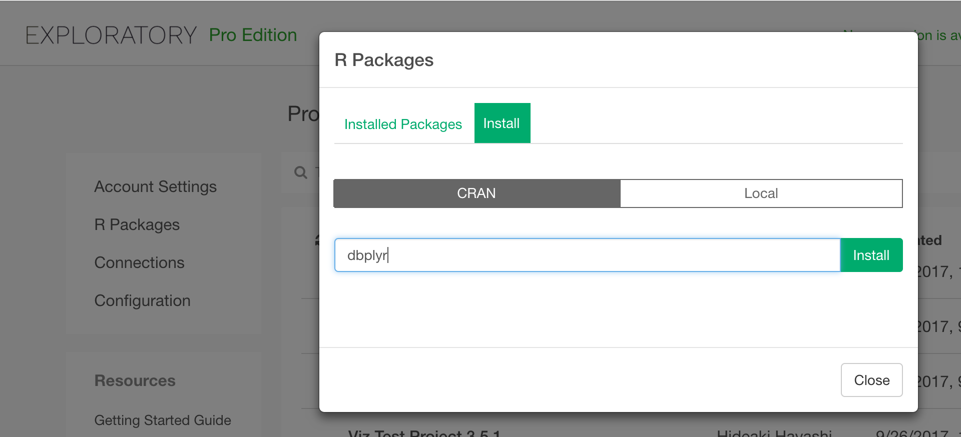
Install dbplyr package

First, you need to install dbplyr package from CRAN to access your database with dplyr,. You can do it inside Exploratory as follows:

Write R Script data source

Then, with Custom R Script data source, you can connect to your Database with dbplyr and dbplyr.

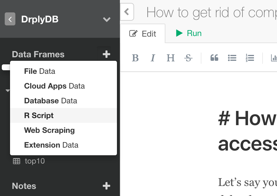
In your custom R Script you can write something like this to connect to your Database (in this example PostgreSQL).

library(dplyr) 

# Connection to Postgres
con <- DBI::dbConnect(RPostgreSQL::PostgreSQL(),    
  host = "localhost",   
  port = 5432,   
  dbname = "postgres",   
  user = "your_user",   
  password = "your_password" )

As a next step, select table airline from the database with the connection you just created.

# Get Table
flights_db <- tbl(con, "airline")

As a starter, let’s write a dplyr query that calculate average departure delay time per origin state.

flights_db %>% 
  group_by(ORIGIN_STATE_ABR) %>% 
  summarize(DEP_DELAY_AVG = mean(DEP_DELAY)) %>%
  collect()

The last collect() is to create a data frame from query result.

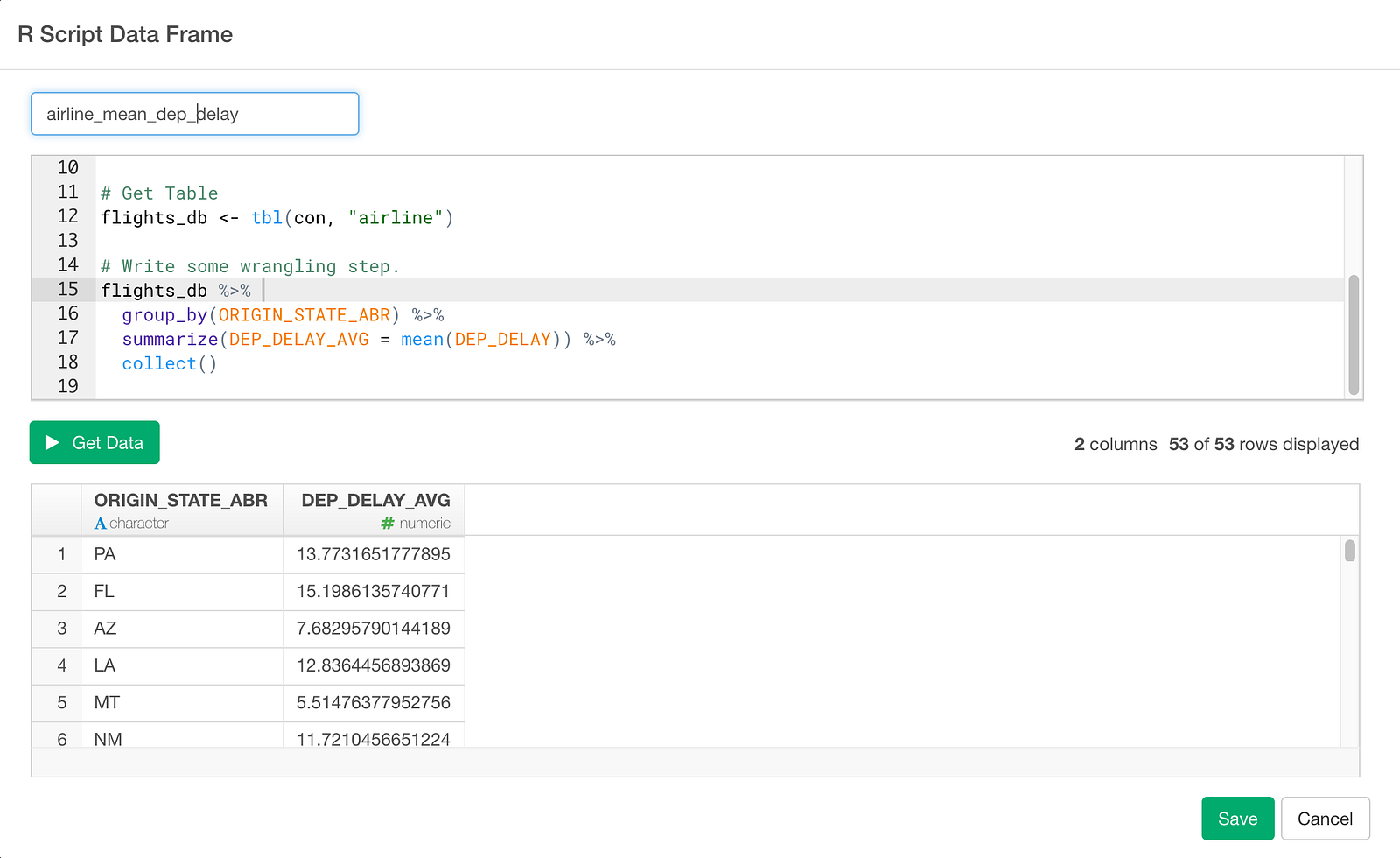
Click Get Data button and check result. If it looks good, click Save button and save as a data frame.

And once it’s saved you can see summary information as follows.

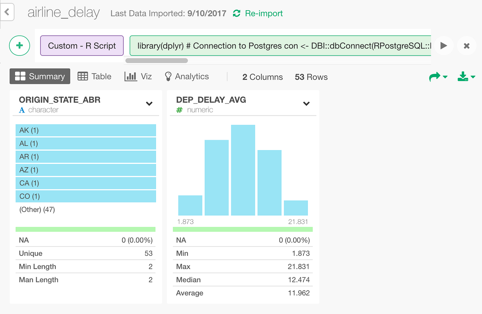
You can also visualize the average departure delay per state on Map like below.

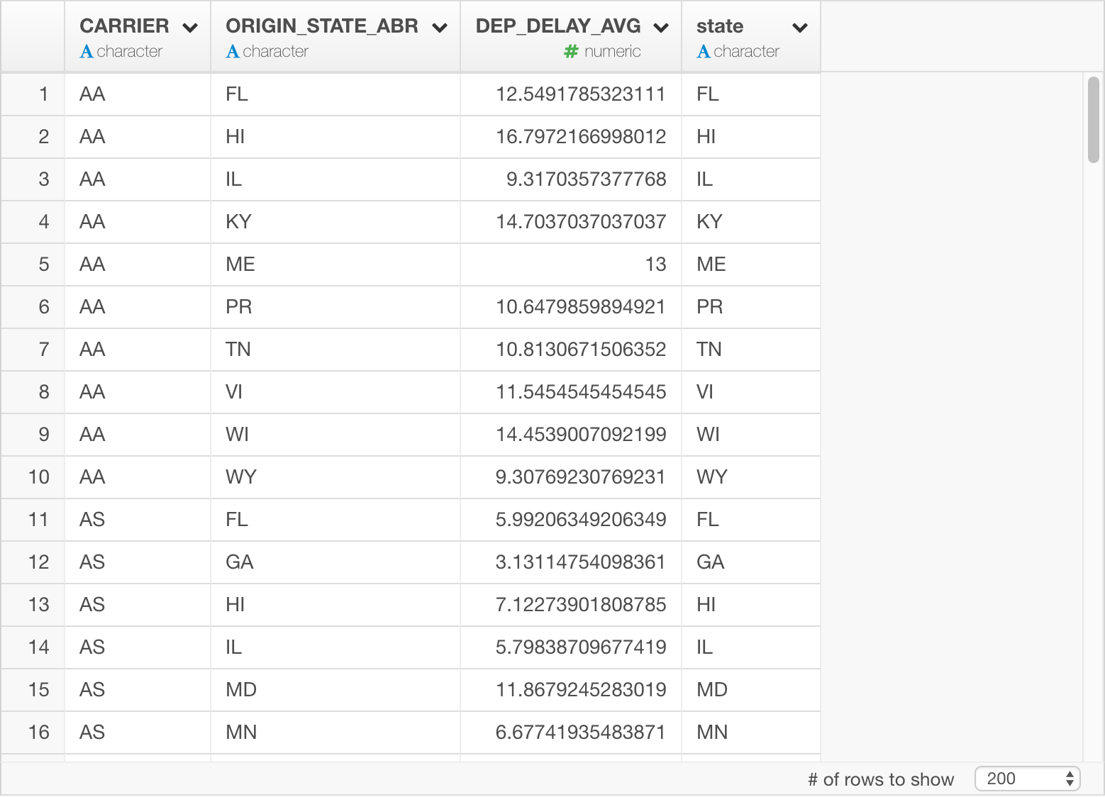
Now, let’s calculate top 10 departure delayed states for each carrier. The dplyr query looks like this.

flights_db %>% 
  group_by(CARRIER, ORIGIN_STATE_ABR) %>% 
  summarize(DEP_DELAY_AVG = mean(DEP_DELAY)) %>%
  top_n(10, DEP_DELAY_AVG) %>%
  collect()

Once you save the data, it looks like this in Exploratory.

By the way, this dplyr query is equivalent of a SQL query like below. You can tell SQL is already getting crazier with the sub-queries.

SELECT "CARRIER", "ORIGIN_STATE_ABR", "DEP_DELAY_AVG"
FROM (SELECT "CARRIER", "ORIGIN_STATE_ABR", "DEP_DELAY_AVG", rank() OVER (PARTITION BY "CARRIER" ORDER BY "DEP_DELAY_AVG" DESC) AS "zzz2"
FROM (SELECT "CARRIER", "ORIGIN_STATE_ABR", AVG("DEP_DELAY") AS "DEP_DELAY_AVG"
FROM "airline"
GROUP BY "CARRIER", "ORIGIN_STATE_ABR") "akblwapghp") "xgqydqtjzm"
WHERE ("zzz2" <= 10.0)

Anyway, I’m visualizing the top 10 states for each Carrier with Bar chart by assigning the states to “X-Axis” and Carrier to “Repeat By”.

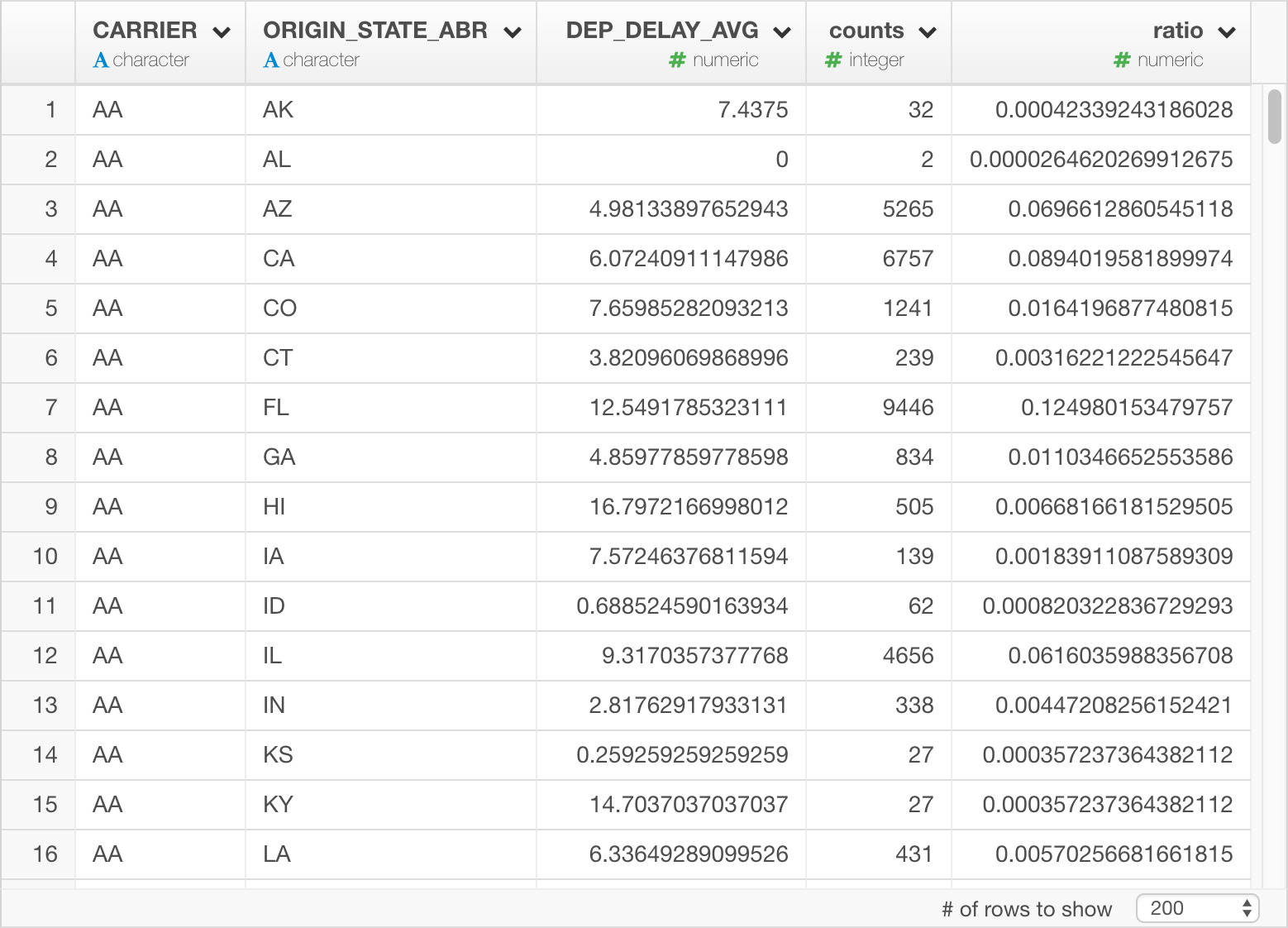
Lastly, for each carrier, let’s calculate average departure delay per state (DEP_DELAY_AVG), number of flights per state (counts), and ratio between number of flights per state and total flights.

flights_db %>% 
 group_by(CARRIER, ORIGIN_STATE_ABR) %>%  
 summarize(DEP_DELAY_AVG = mean(DEP_DELAY), counts = n()) %>% 
 mutate(ratio = counts/sum(counts)) %>%
 collect()

Once you save the result, it looks like this.

Here’s an equivalent of SQL query… Just in case…

SELECT "CARRIER", "ORIGIN_STATE_ABR", "DEP_DELAY_AVG", "counts", "counts" / sum("counts") OVER (PARTITION BY "CARRIER") AS "ratio"
FROM (SELECT "CARRIER", "ORIGIN_STATE_ABR", AVG("DEP_DELAY") AS "DEP_DELAY_AVG", count(*) AS "counts"
FROM "airline"
GROUP BY "CARRIER", "ORIGIN_STATE_ABR") "zovxinlfni"

Now I’m visualizing the result with bar chart by assigning Carrier to X-Axis and State to color.

Summary

By leveraging dbplyr and dplyr with Exploratory, you can work with database data effectively without a need of writing complex SQL queries. And this improves not only your productivity but also others you share your analysis works with. It’s a Win-Win!

If you don’t have Exploratory Desktop yet, you can sign up from here for a 30 days free trial. If you are currently a student or teacher, then it’s free!