Accessing SQLite with RSQLite and Querying with dplyr in R Script

SQLite is an embedded SQL database engine. SQLite reads and writes directly to ordinary disk files and the database file format is cross-platform - you can freely copy a database between 32-bit and 64-bit systems or between big-endian and little-endian architectures. So thanks to this compactness and portability, there are many data available in SQLite format. For example, if you go to this Kaggle site, you can see Japan’s international trade by country and type of good Data as SQLite data files.

Anyway, in this post, I’m going to walk you through how you can use RSQLite and dplyr to query and get results directly from the SQLite data quickly.

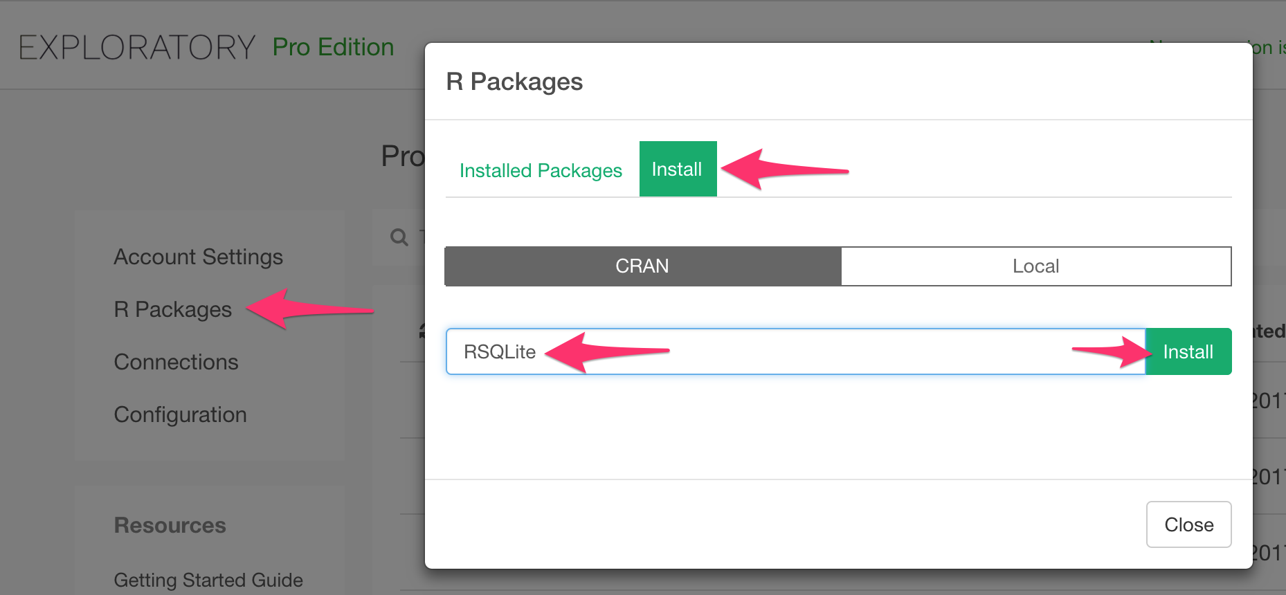
Install RSQLite package

First, you need to install RSQLite package from CRAN to access your database with dplyr,. You can do it inside Exploratory as follows:

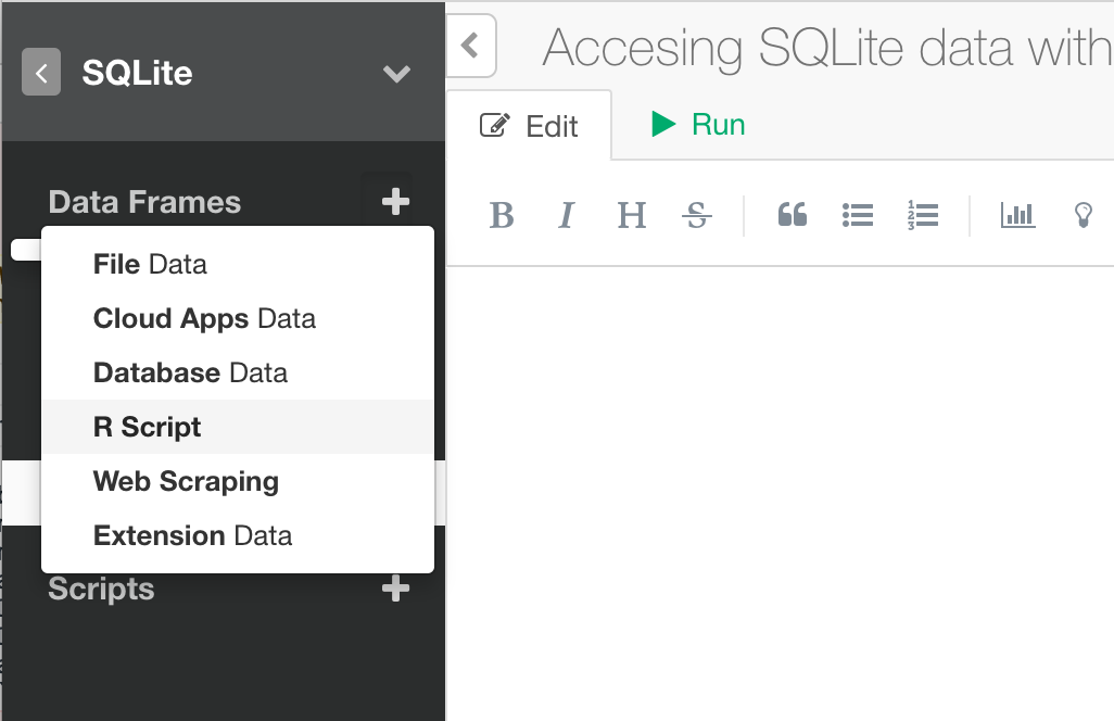
Write R Script data source

Then, after you downloaded SQLite data from Kaggle, with Custom R Script data source, you can access your SQLite Database with RSQLite.

In your custom R Script you can write something like this to connect to your SQLite Database. As you would guess, /Users/hidekoji/Downloads/year_1988_2015.db is the SQLite file that I downloaded from the Kaggle.

library(DBI)
library(RSQLite)
con <- dbConnect(SQLite(), "/Users/hidekoji/Downloads/year_1988_2015.db")

As a next step, select table year_1988_2015 from the database with the connection you just created.

# Get table
year_1988_2015 <- dbReadTable(con2015, 'year_1988_2015')

As a starter, let’s write a dplyr query that calculate total traded amount (from 1988 to 2015) for each country.

# data is fetched so disconnect it.
dbDisconnect(con)

# Cancluate Total trade amount per country
year_1988_2015 %>% group_by(Country) %>% 
summarize(total_vy = sum(VY))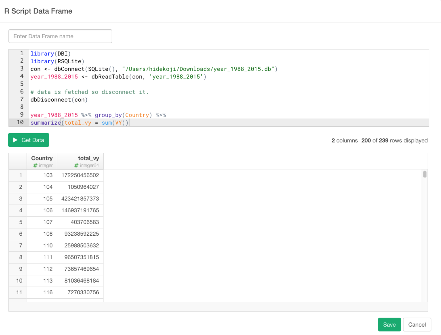

Click Get Data button and check result. If it looks good, click Save button and save as a data frame.

And once it’s saved you can see summary information as follows.

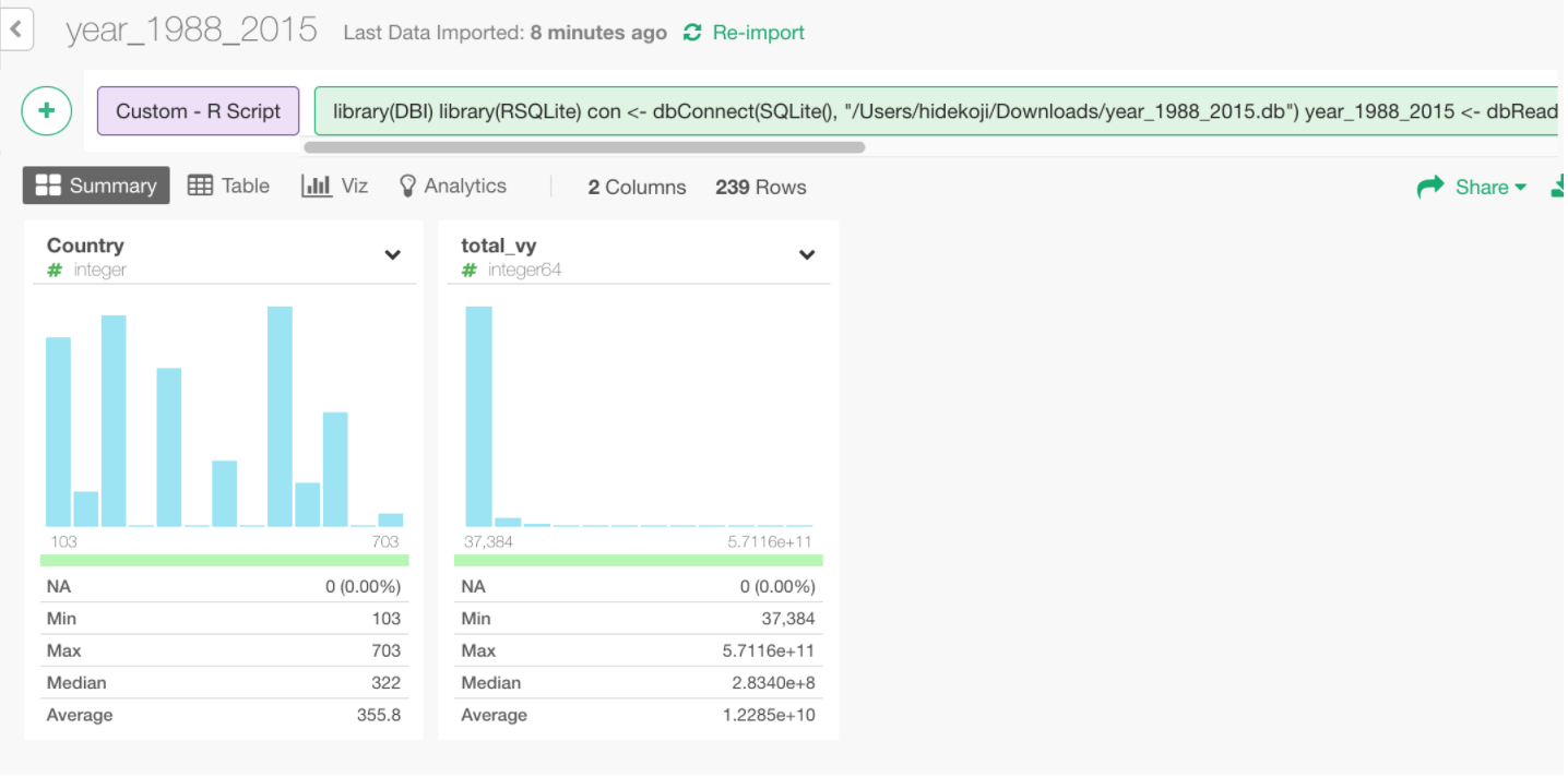
It seems Country column hodls country code instead of name, so let’s get a country name mapping csv fle from Kaggle too.

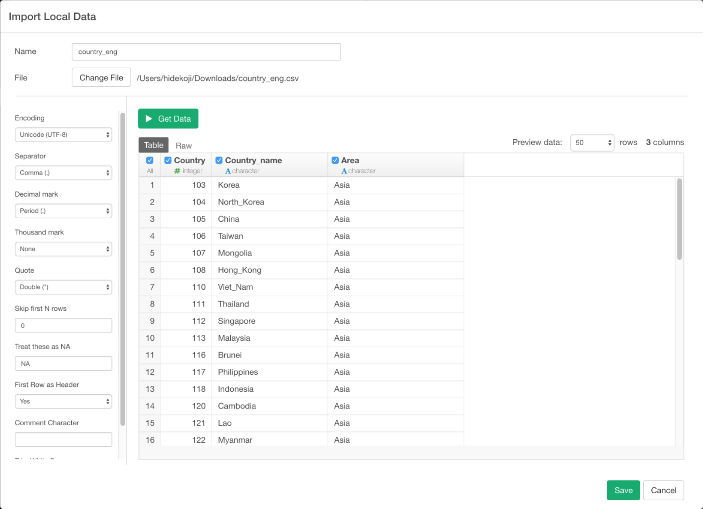
Once you load it, join country_eng table with year_1988_2015 table.

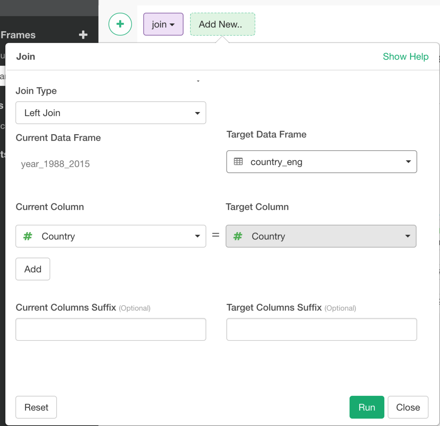
Now you can see each country name.

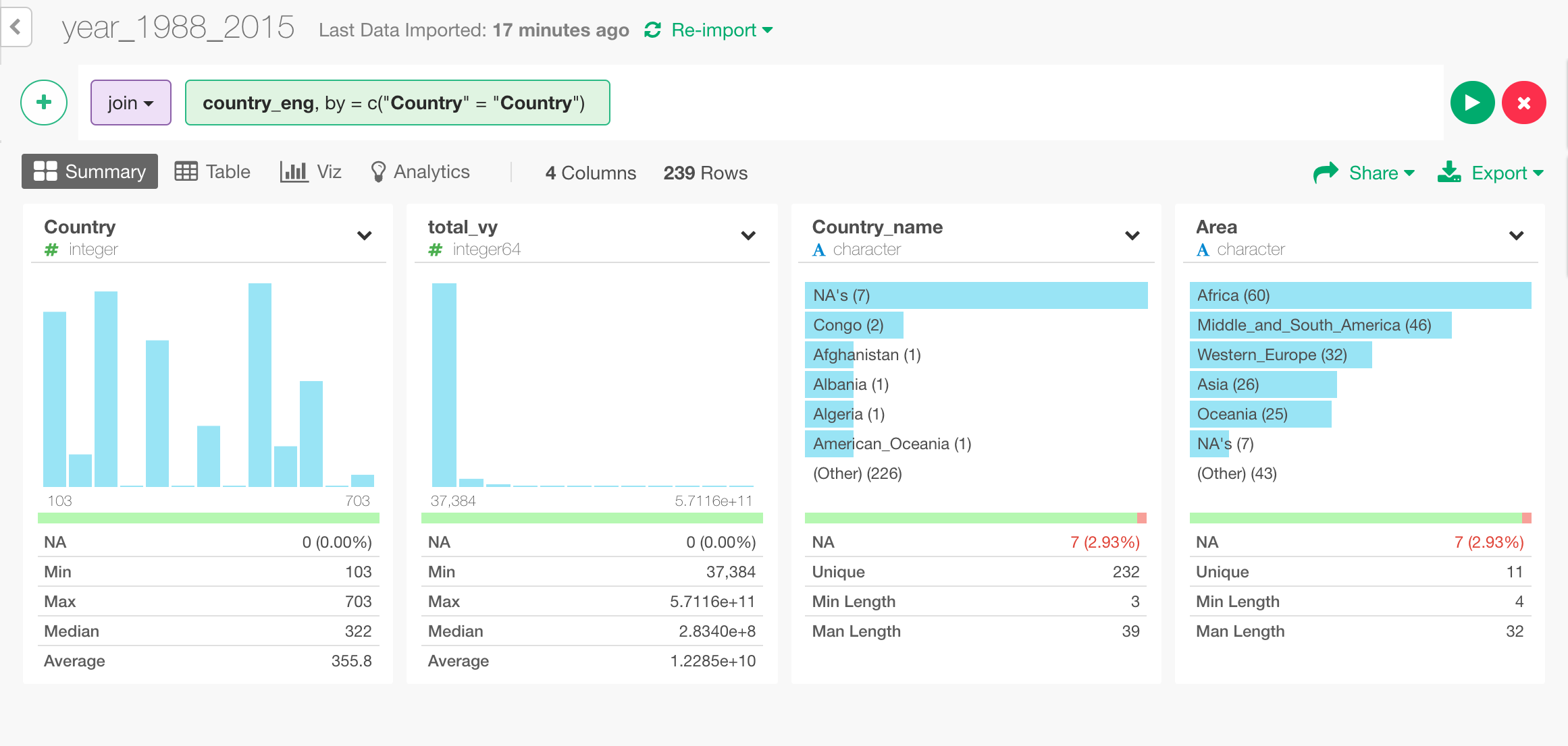
Since the Country Name is connected with underscore like United_States_of_America, we wanto to replace underscore _ with space so that we can project them on World Map.

To do this, we can use Replace All under Work with Text menu.

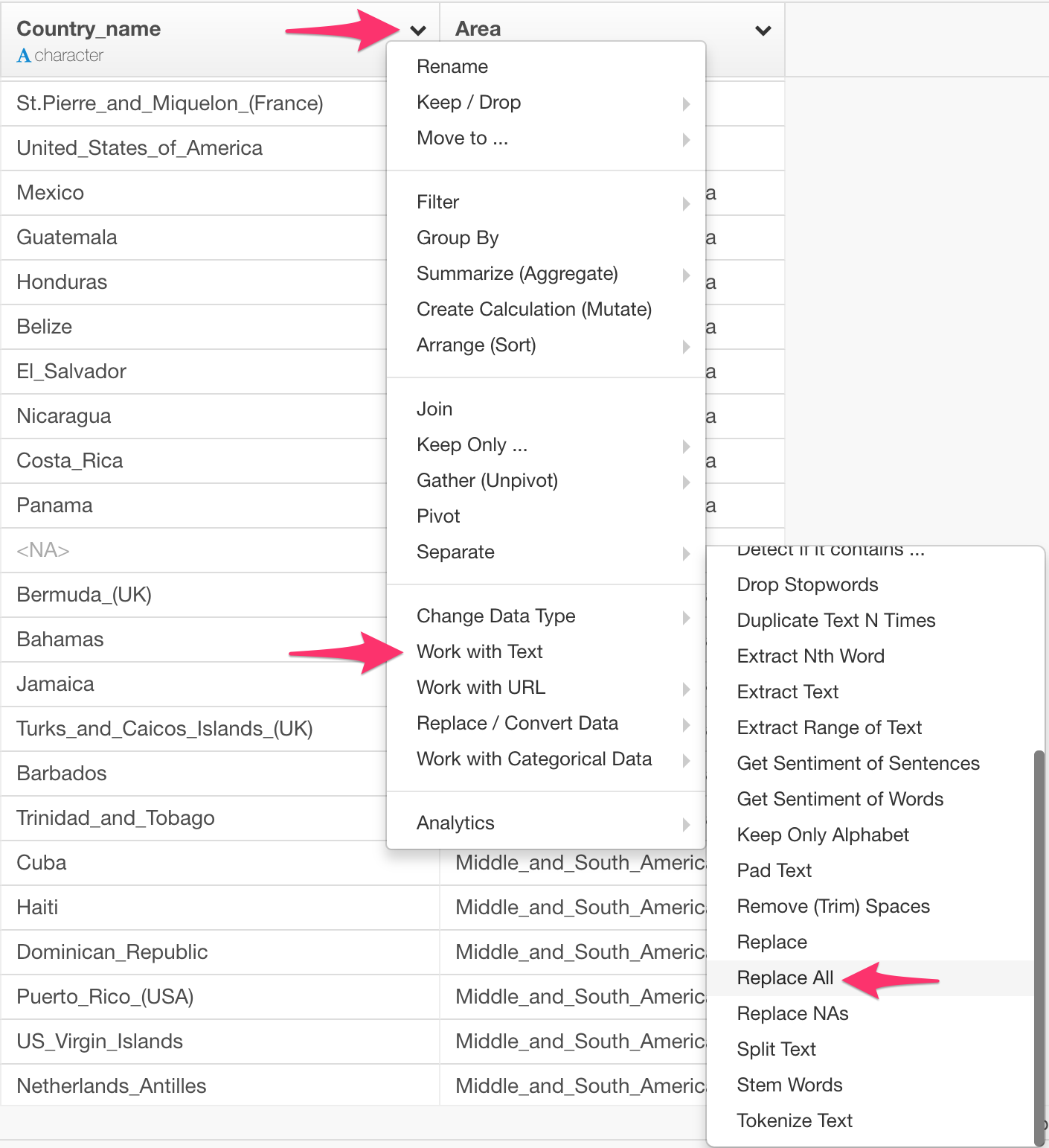
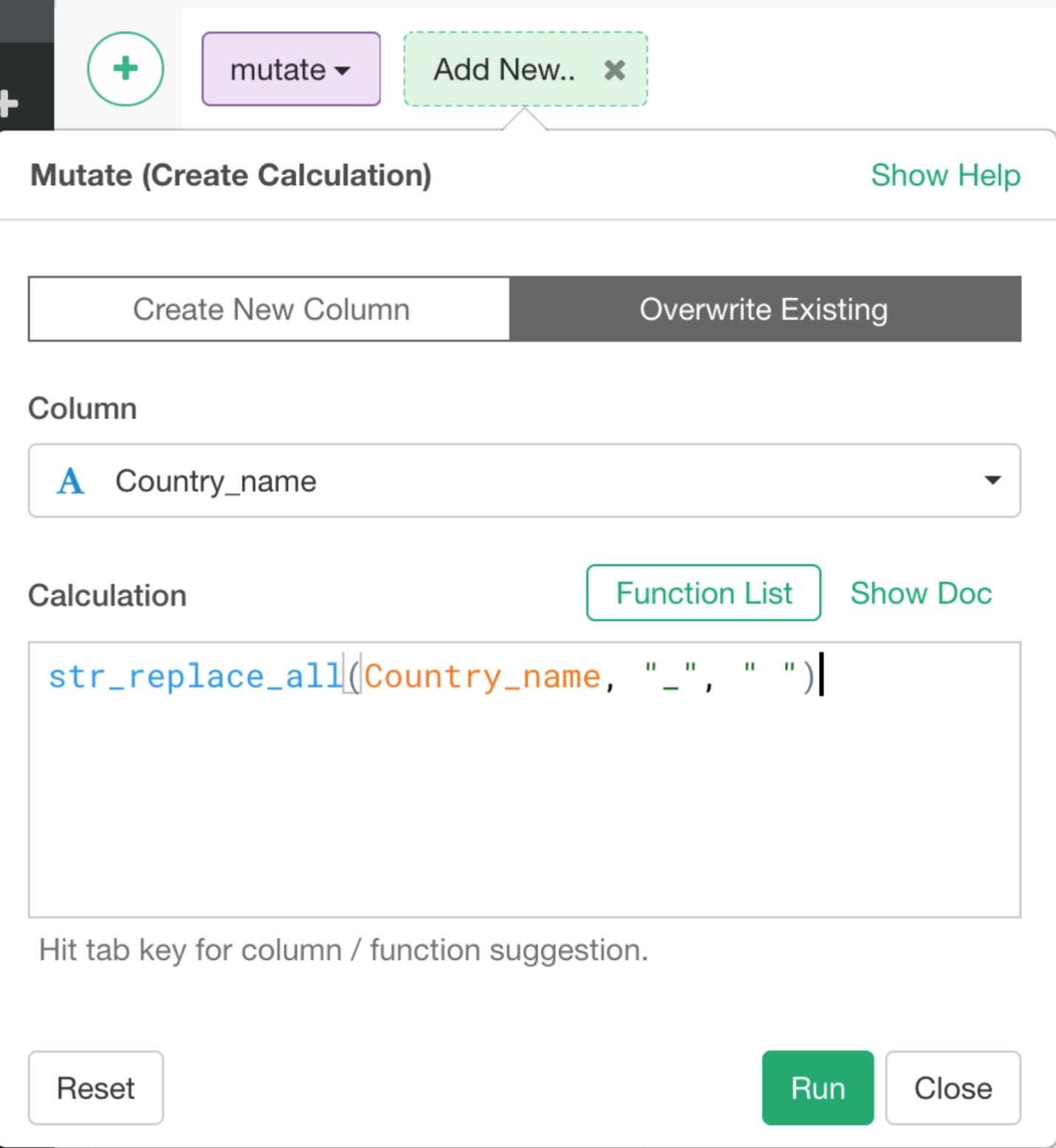
And pass _ as second argument and " " as third argument so that all the _ are replaced with " ".

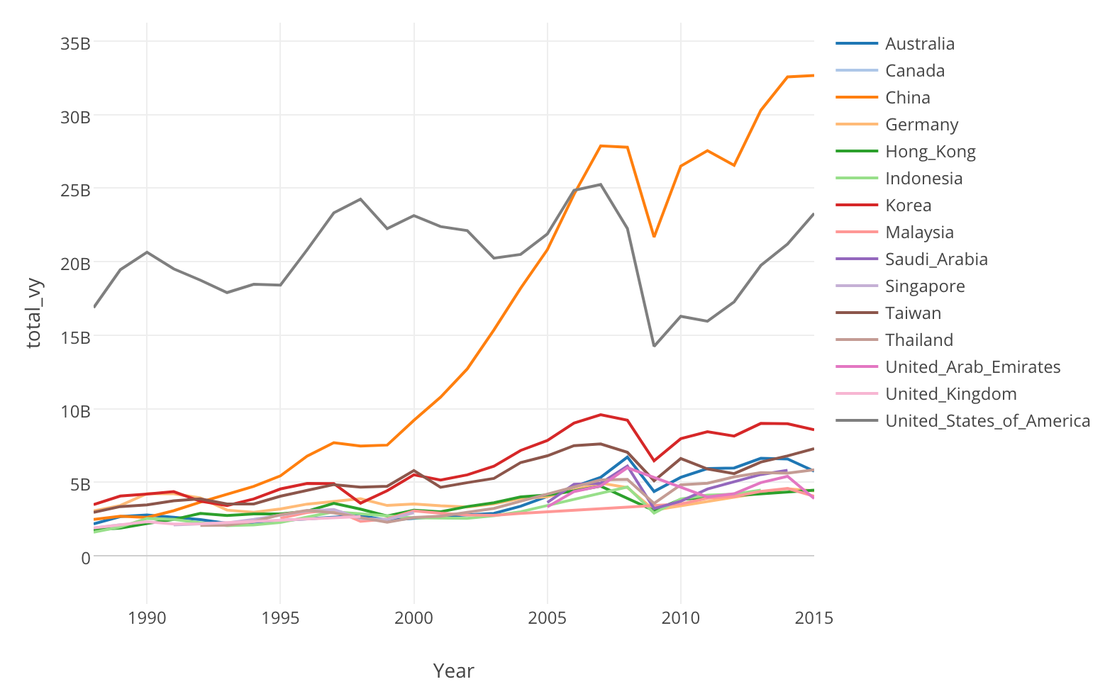
You can visualize the Japan’s total traded amount per trading country on Map like below. And we can see Japan has been doing lot of export/import with US and China.

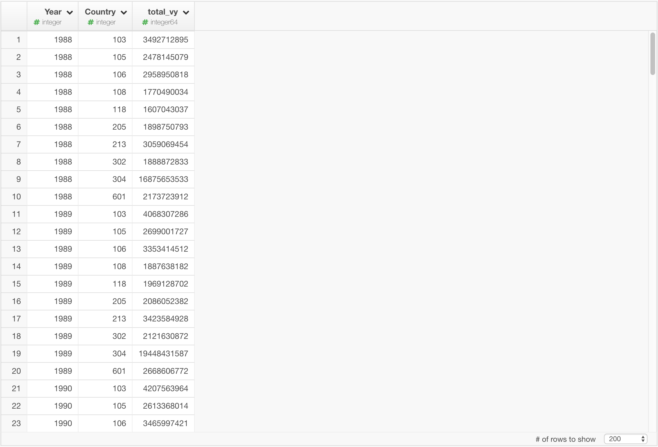
Now, for each year, let’s calculate top 10 countries that Japan has been doing business with. The dplyr query looks like this.

year_1988_2015 %>% group_by(Year, Country) %>% 
summarize(total_vy = sum(VY)) %>%
top_n(10, total_vy)

Once you save the data, it looks like this in Exploratory.

Anyway, after joining it the country table, I’m visualizing the top 10 countries for each Year with Line chart by assigning the Year to “X-Axis” and CountryName as “Color By”. And now you can see how China has rapidly increased trading with Japan and took #1 country position in 2007 from United States.

Summary

By leveraging RSQLite and dplyr with Exploratory, you can work with SQLite database data effectively without a need of writing complex SQL queries. And this improves not only your productivity but also others you share your analysis works with. It’s a Win-Win!

I shared the data in EDF (Exploratory Data Format) so that you can import it and test it on your Exploratory Desktop.

If you don’t have Exploratory Desktop yet, you can sign up from here for a 30 days free trial. If you are currently a student or teacher, then it’s free!