Building Deep Learning Models with Keras inside Exploratory

Install and Setup

We want to install ‘keras’ R package, install Keras itself, and setup Keras inside Exploratory.

1. Install ‘keras’ package

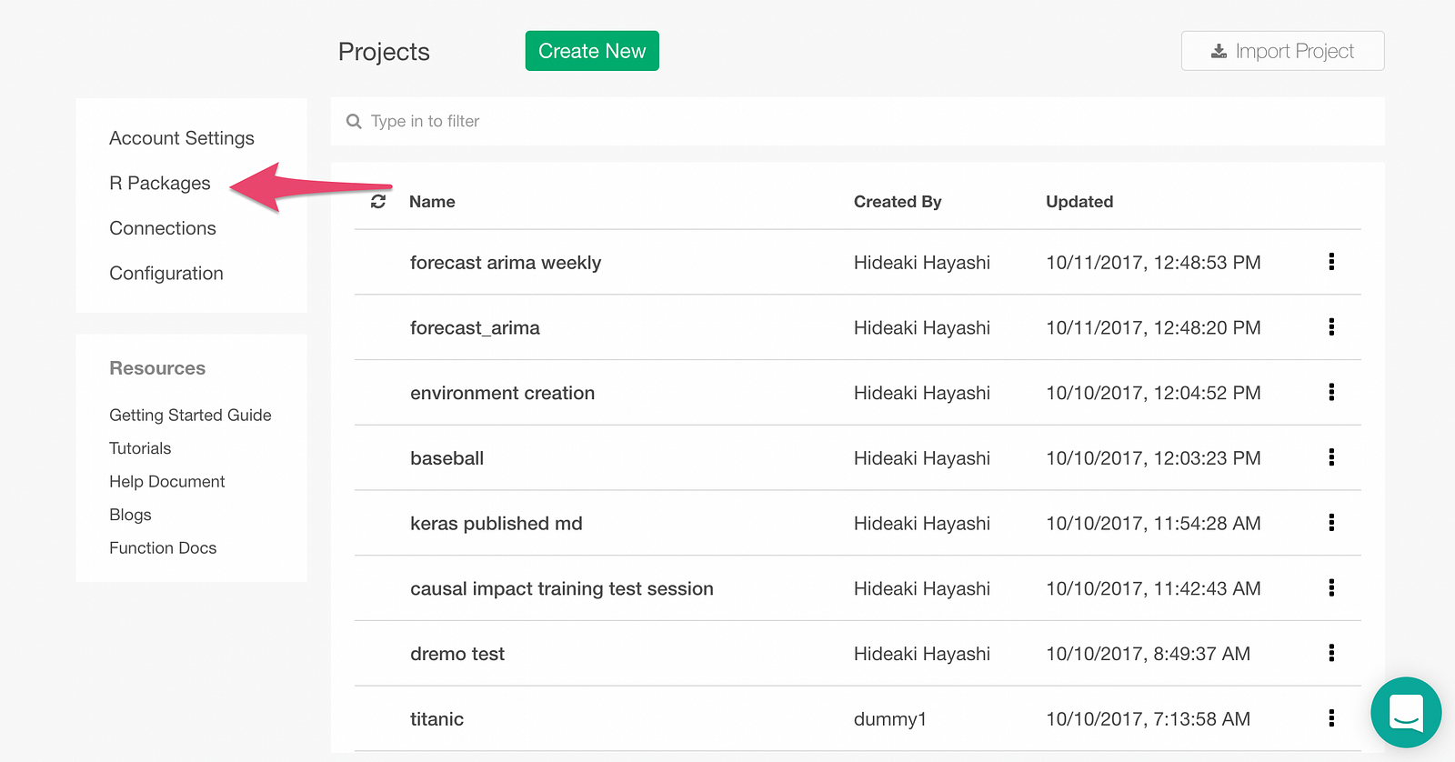
From the lefthand-side menu on the Project List page, select “R Packages”

On the R Packages Dialog, type in “keras” and click Install.

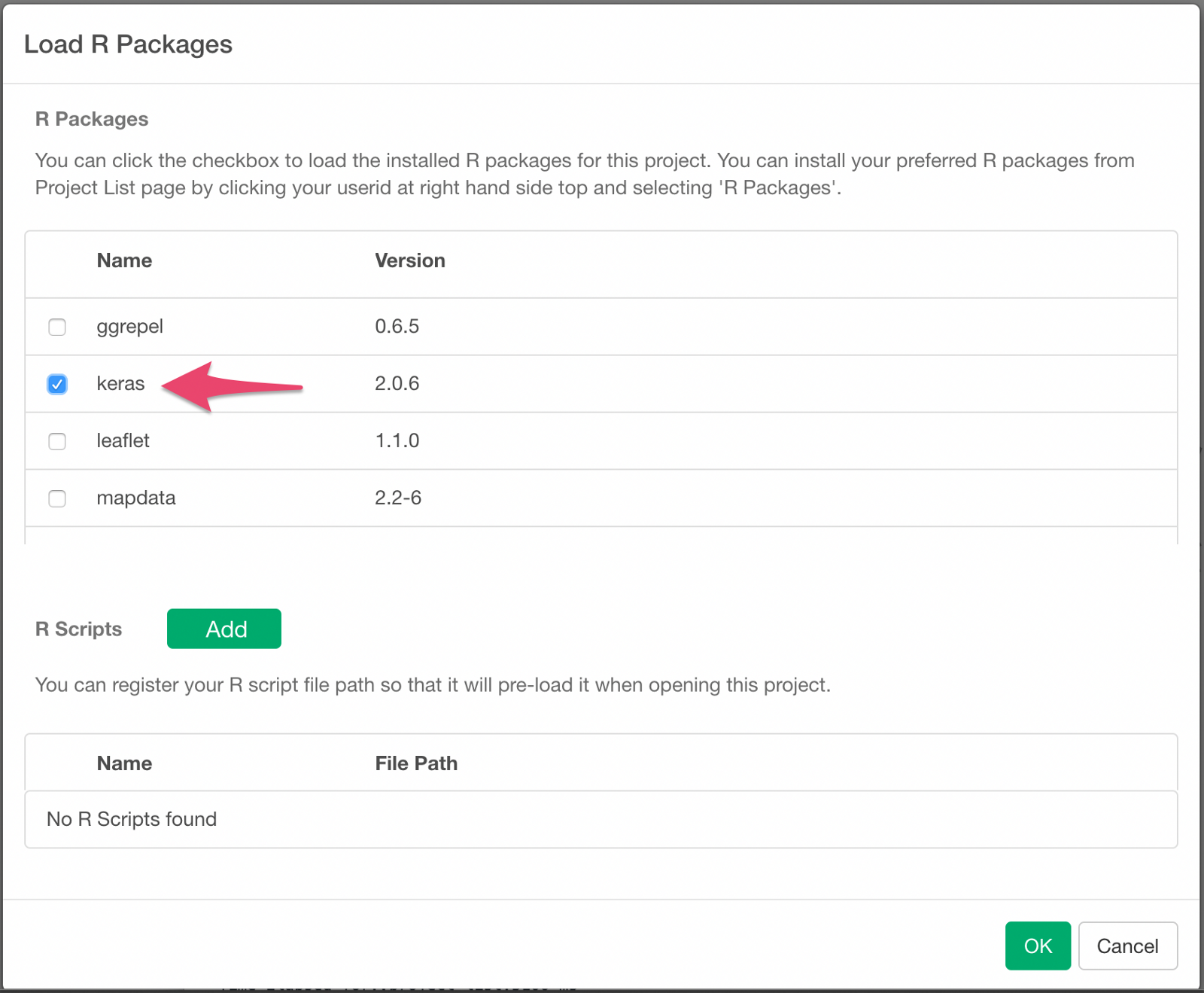
Once it’s installed, open an project and find R Package menu like below and click on it.

Image file not found: /Users/hideaki/.exploratory/projects/keras4_a09287225533/markdown_output/image-1528758065031.png

Check the checkbox for keras package to load the package every time you open this project.

Install keras backend

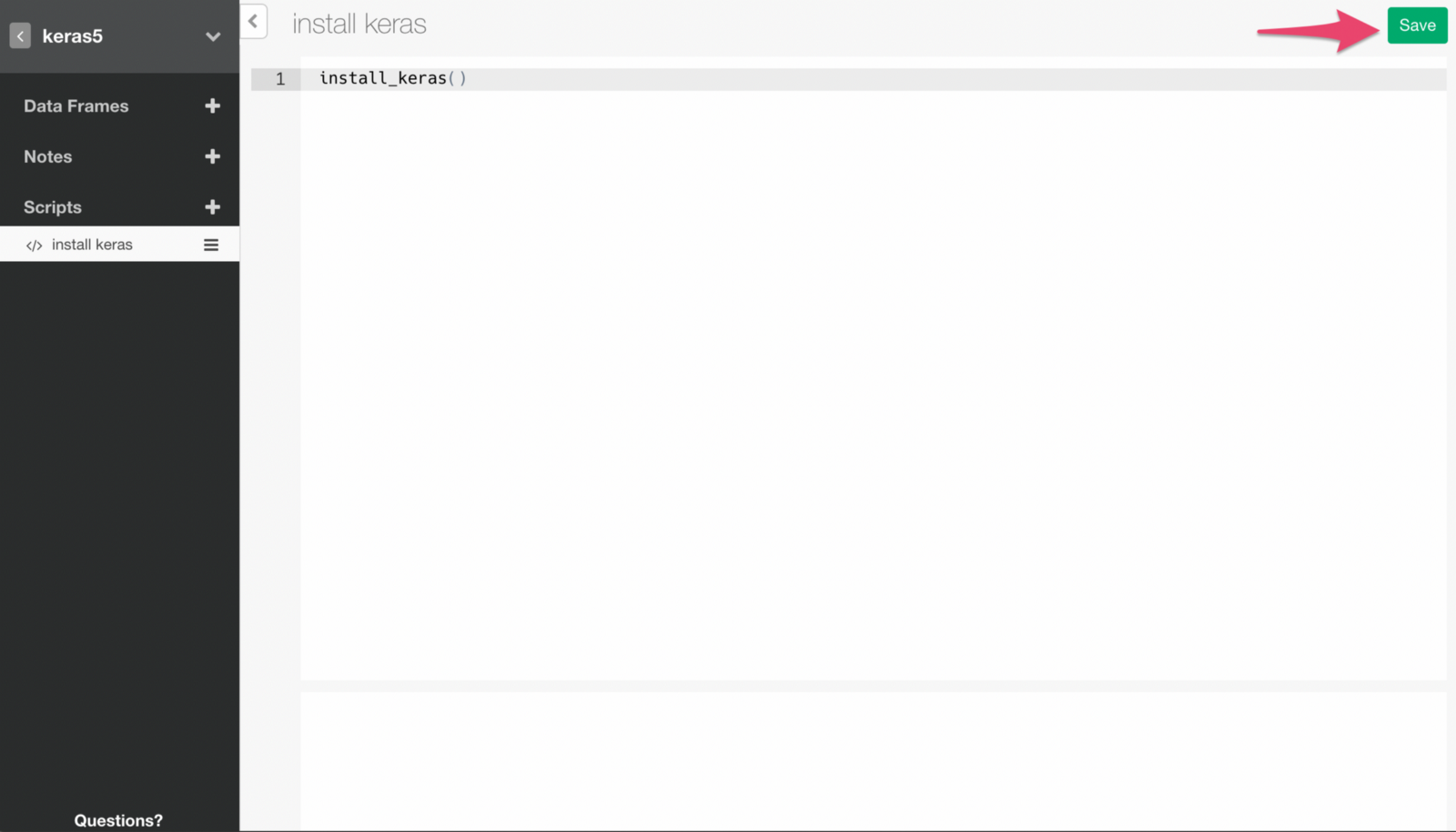
Create a Script by clicking + (plus) icon next to Scripts menu and typing in the name for the new Script.

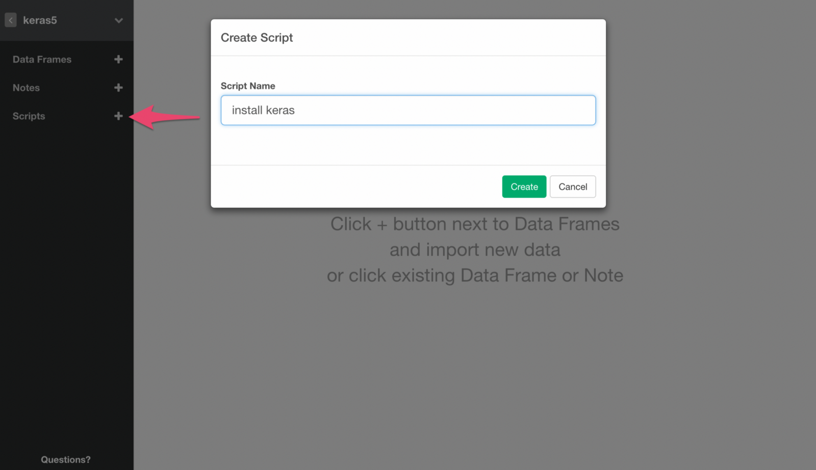
Copy the following command in it. It installs the backend of keras package.

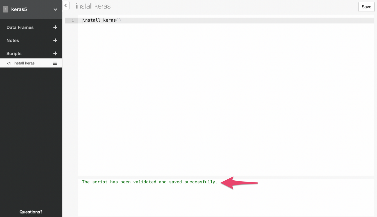
install_keras()

Run the command by clicking Save button.

If the command runs successfully, you will see a message like below.

Note that you only need to run this command once. This means we want to make sure to remove this script at this point, otherwise it will run and try to install Keras every time you open the project, which you don’t want to.

Setup Keras with Exploratory’s Model Extension Framework

In Exploratory, many machine learning models are already supported out-of-the-box with its UI, but you can add other models you want to use by writing Custom R Scripts for Exploratory’s Model Extension Framework.

• How to add custom model

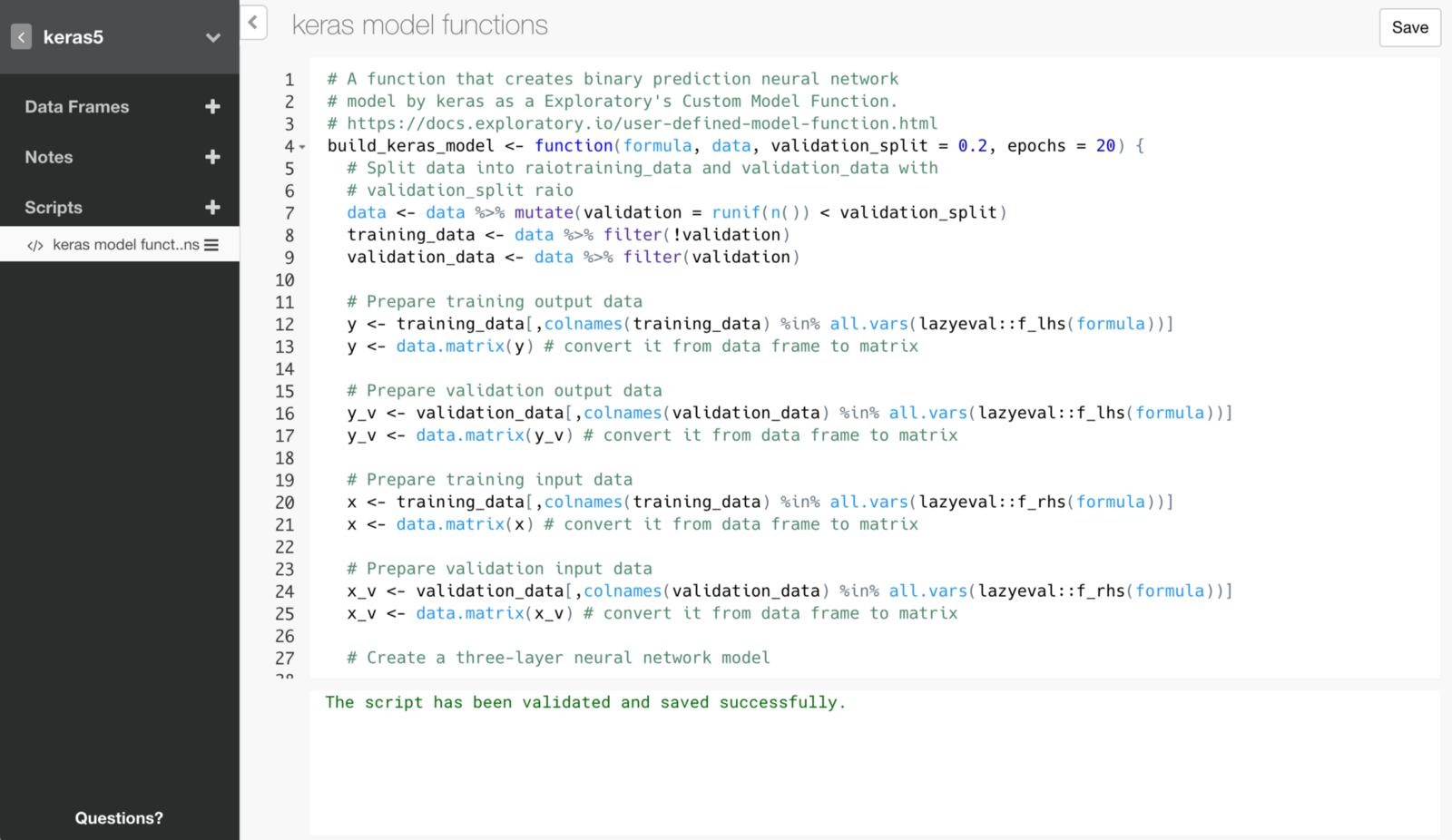
Here is an R script that makes use of the framework to build Deep Learning models with Keras inside Exploratory.

# A function that creates binary prediction neural network 
# model by keras as a Exploratory's Custom Model Function.
# https://docs.exploratory.io/user-defined-model-function.html
build_keras_model <- function(formula, data, validation_split = 0.2, epochs = 20) {
  # Split data into raiotraining_data and validation_data with
  # validation_split raio
  data <- data %>% mutate(validation = runif(n()) < validation_split)
  training_data <- data %>% filter(!validation)
  validation_data <- data %>% filter(validation)
  
  # Prepare training output data
  y <- training_data[,colnames(training_data) %in% all.vars(lazyeval::f_lhs(formula))]
  y <- data.matrix(y) # convert it from data frame to matrix
  
  # Prepare validation output data
  y_v <- validation_data[,colnames(validation_data) %in% all.vars(lazyeval::f_lhs(formula))]
  y_v <- data.matrix(y_v) # convert it from data frame to matrix
  
  # Prepare training input data
  x <- training_data[,colnames(training_data) %in% all.vars(lazyeval::f_rhs(formula))]
  x <- data.matrix(x) # convert it from data frame to matrix
  
  # Prepare validation input data
  x_v <- validation_data[,colnames(validation_data) %in% all.vars(lazyeval::f_rhs(formula))]
  x_v <- data.matrix(x_v) # convert it from data frame to matrix

  # Create a three-layer neural network model

  model <- keras_model_sequential() 
  model %>% 
    layer_dense(units = 7, activation = 'relu', input_shape = c(7)) %>% # set 7 neurons in the first layer
    layer_dropout(rate = 0.2) %>% # dropout 20% of the data
    layer_dense(units = 5, activation = 'relu') %>% # set 5 neurons in the second layer
    layer_dropout(rate = 0.1) %>% # dropout 10% of the data
    layer_dense(units = 1, activation = 'sigmoid') # Summarize them as a one survival probability in the third layer
  
  model %>% compile(
    loss = loss_binary_crossentropy,
    optimizer = optimizer_adam(),
    metrics = c('accuracy')
  )

  # Train model with training data.
  history <- model %>% fit(
    x, y, 
    epochs = epochs, batch_size = 20,
    validation_data = list(x_v, y_v),
    verbose = 0
  )
  
  # Return model, history, and forumala as a single object
  ret <- list(model = model, history=history, formula = formula)
  class(ret) <- c("keras_model")
  ret
}

# A function to predict with trained model and new data
augment.keras_model <- function(x, data = NULL, newdata = NULL, ...) {
  formula <- x$formula
  if (is.null(data)) {
    data <- newdata
  }
  data_x <- data[,colnames(data) %in% all.vars(lazyeval::f_rhs(formula))]
  data_x <- data.matrix(data_x)
  y <- x$model %>% predict_proba(data_x)
  ret <- data
  ret$y <- as.numeric(y)
  ret
}

# A function to extract information for model summary view as a data frame from the model
glance.keras_model <- function(x, ...){
  params <- x$history$params
  params$metrics <- NULL
  params$steps <- NULL
  as.data.frame(params)
}

# Another function to extract information for model summary view as a data frame from the model
# pritn history info
tidy.keras_model <- function(x, ...){
  as.data.frame(x$history)
}

You can create a new script and copy/paste the code above, and click Save button to run and save it.

Importing and Preparing Data

Import Data

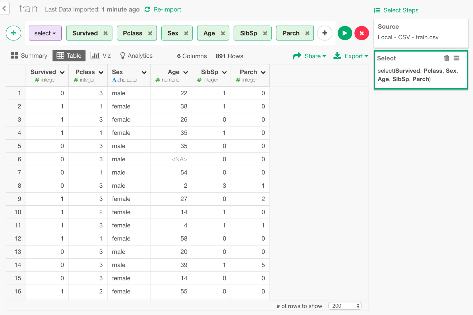
Download the Titanic’s training data called train.csv from here and import it into Exploratory.

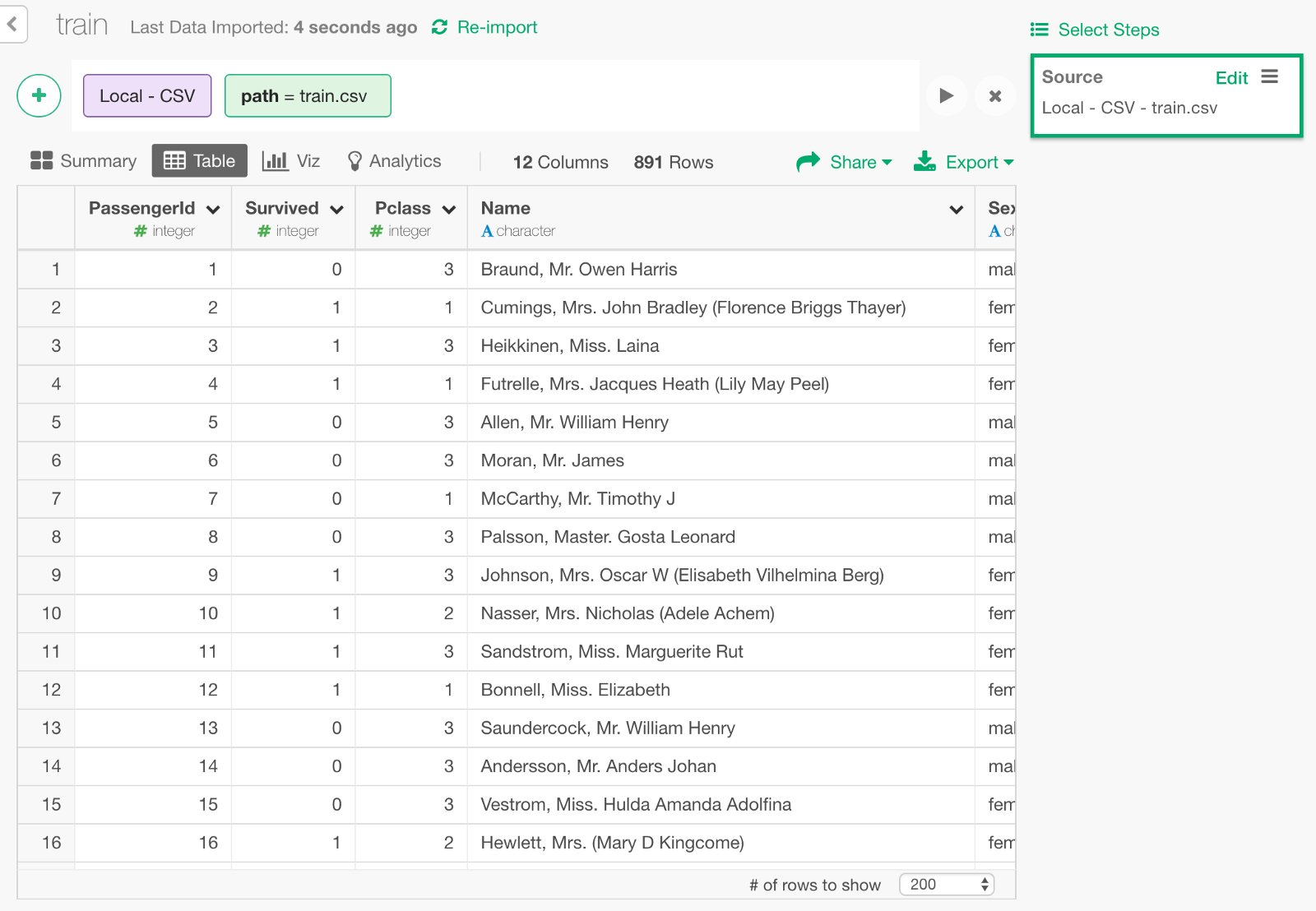
We can keep only the following columns that we need to build a model.

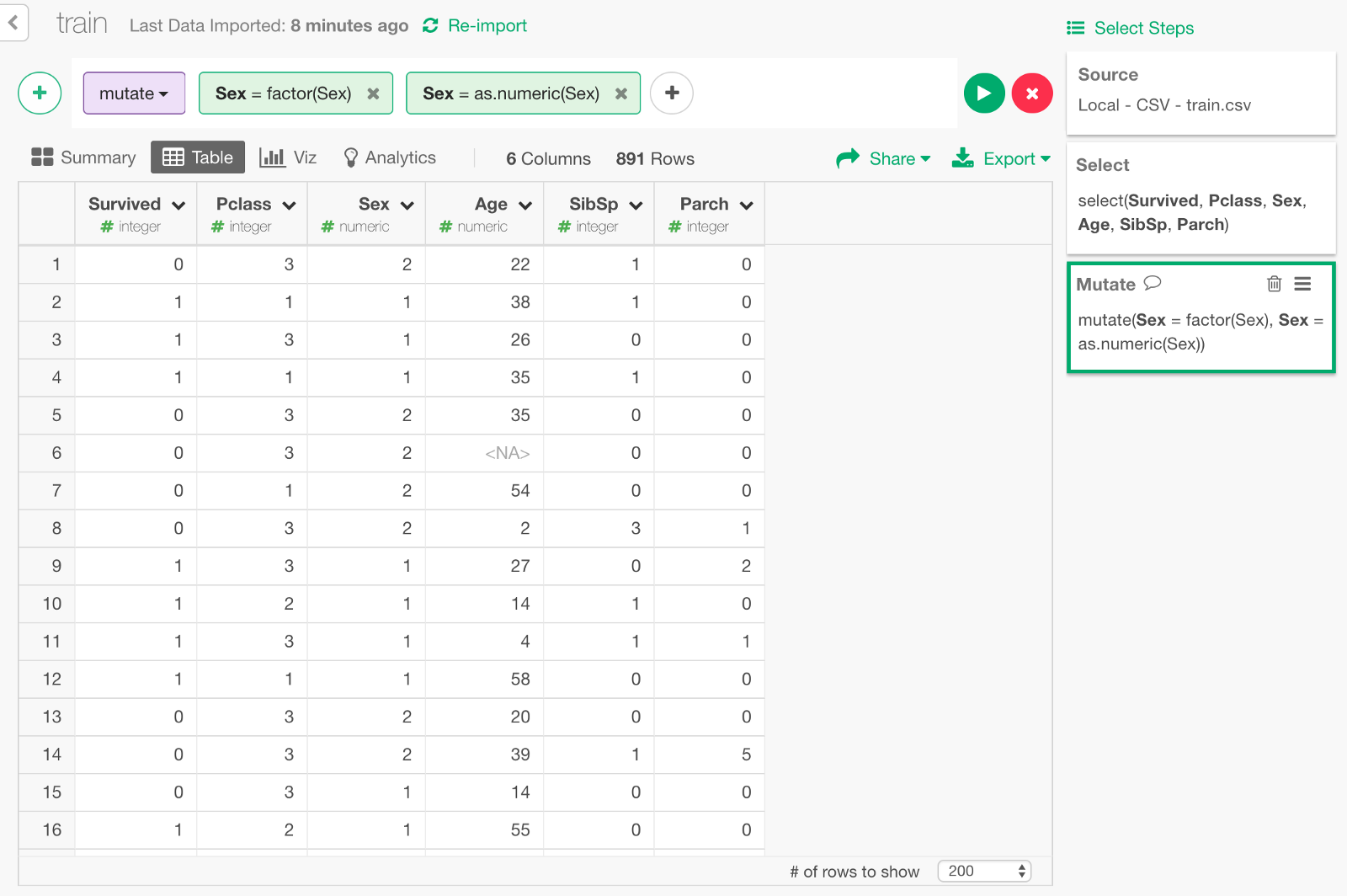
Convert gender data to numeric

All the predictor columns need to be numeric data type for the Deep Learning model of keras. This means that we need to transform ‘Sex’ column by converting ‘male’ or ‘female’ to 1 and 2 respectively. We can convert it as Factor data type first, then convert it as numeric as follows.

Normalize Age

Another thing is, columns other than Age are all within the range of single digit numbers such as 1 or 2, but Age is scaled from 0 to 80. In order to improve learning performance, it is commonly advised to normalize the distribution of input parameters. Let’s do it by using normalize function in exploratory package. (Since keras also has a function called normalize, we call the function as exploratory :: normalize to distinguish it.)

exploratory::normalize(Age)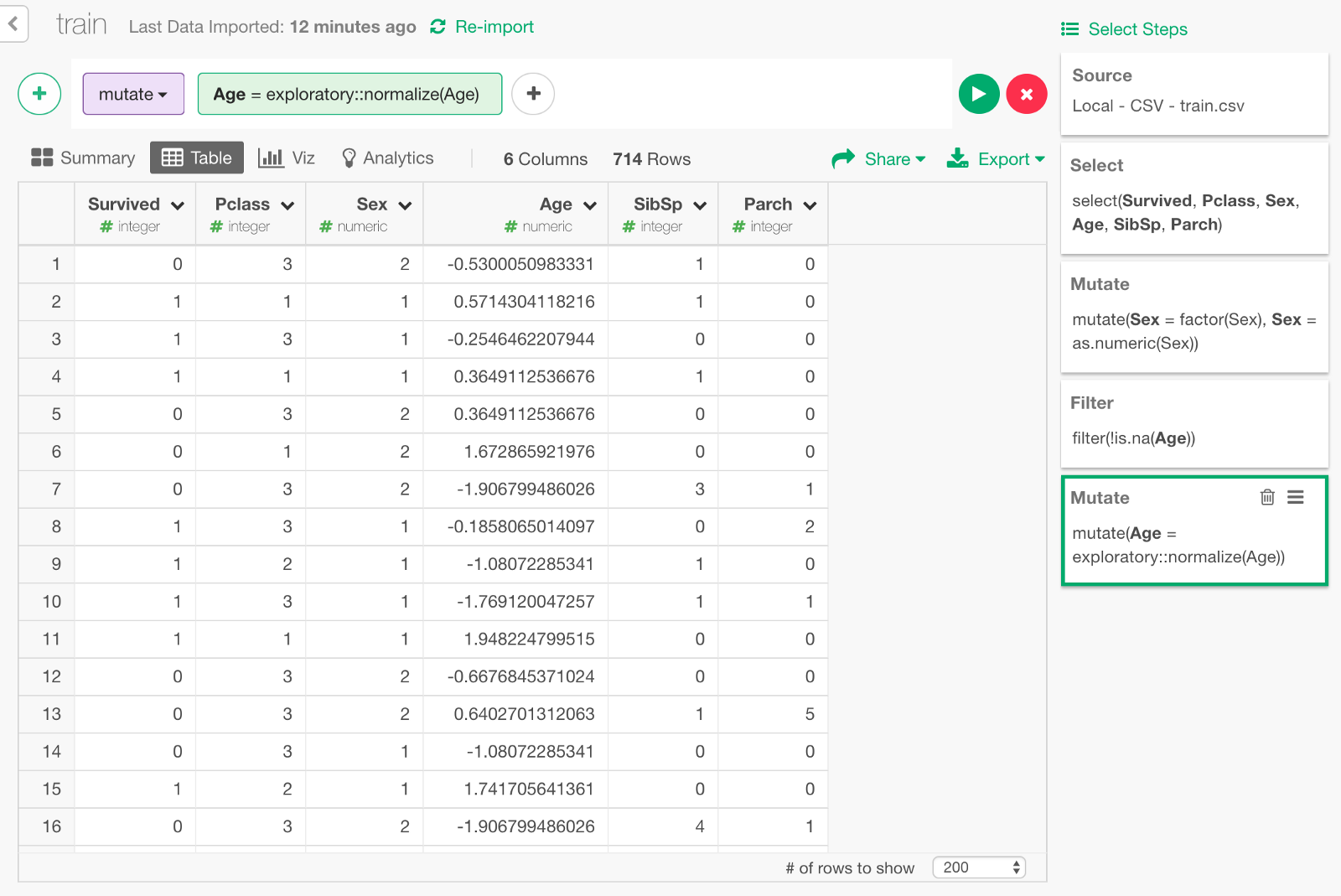

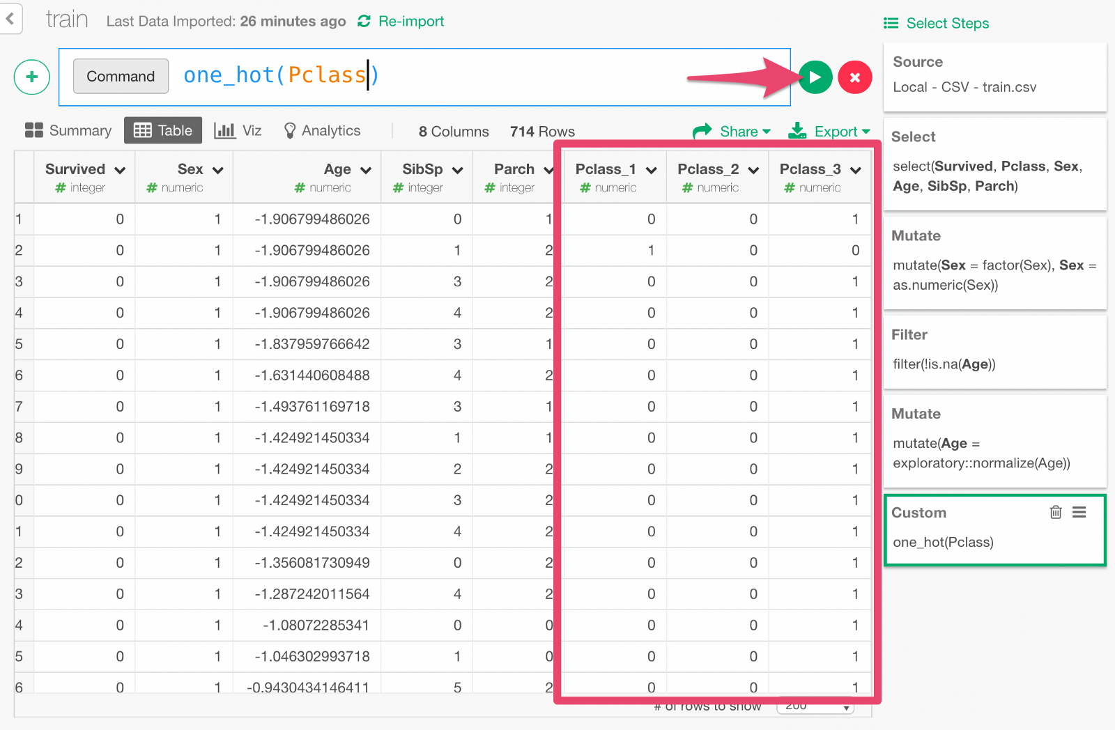
One-Hot Encoding of boarding ticket type

Pclass (boarding ticket type) column is numerical, but we want to treat it as category for this exercise. Since the Deep Learning model of Keras can’t handle categorical columns, we can create ‘dummy’ columns, each of which represents each of the categorical value of Pclass and has 0 or 1 based on whether it matches or not. This is commonly called one-hot encoding.

I have prepared a function named one_hot to do this. Create a Script and copy the following, so that we can use it in Exploratory.

# A utility function for One-hot encoding
one_hot <- function(df, key) {
  key_col <- dplyr::select_var(names(df), !! rlang::enquo(key))
  df <- df %>% mutate(.value = 1, .id = seq(n()))
  df <- df %>% tidyr::spread_(key_col, ".value", fill = 0, sep = "_") %>% select(-.id)
}

Now, let’s make a custom command step to call this function.

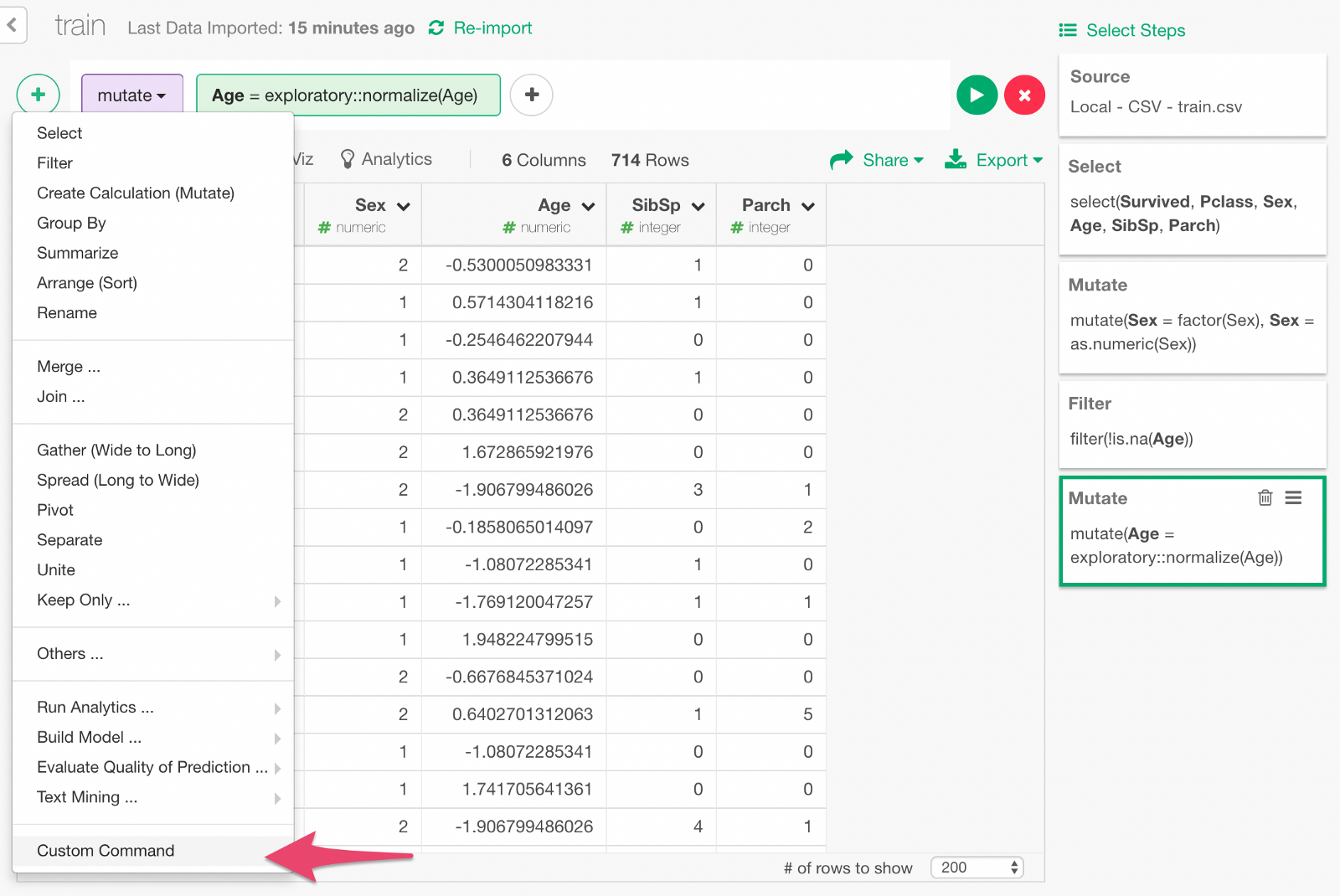
Type in the custom command. Click Run button, and you will see a set of new columns as the result of one-hot encoding.

Build Deep Learning Model with Keras

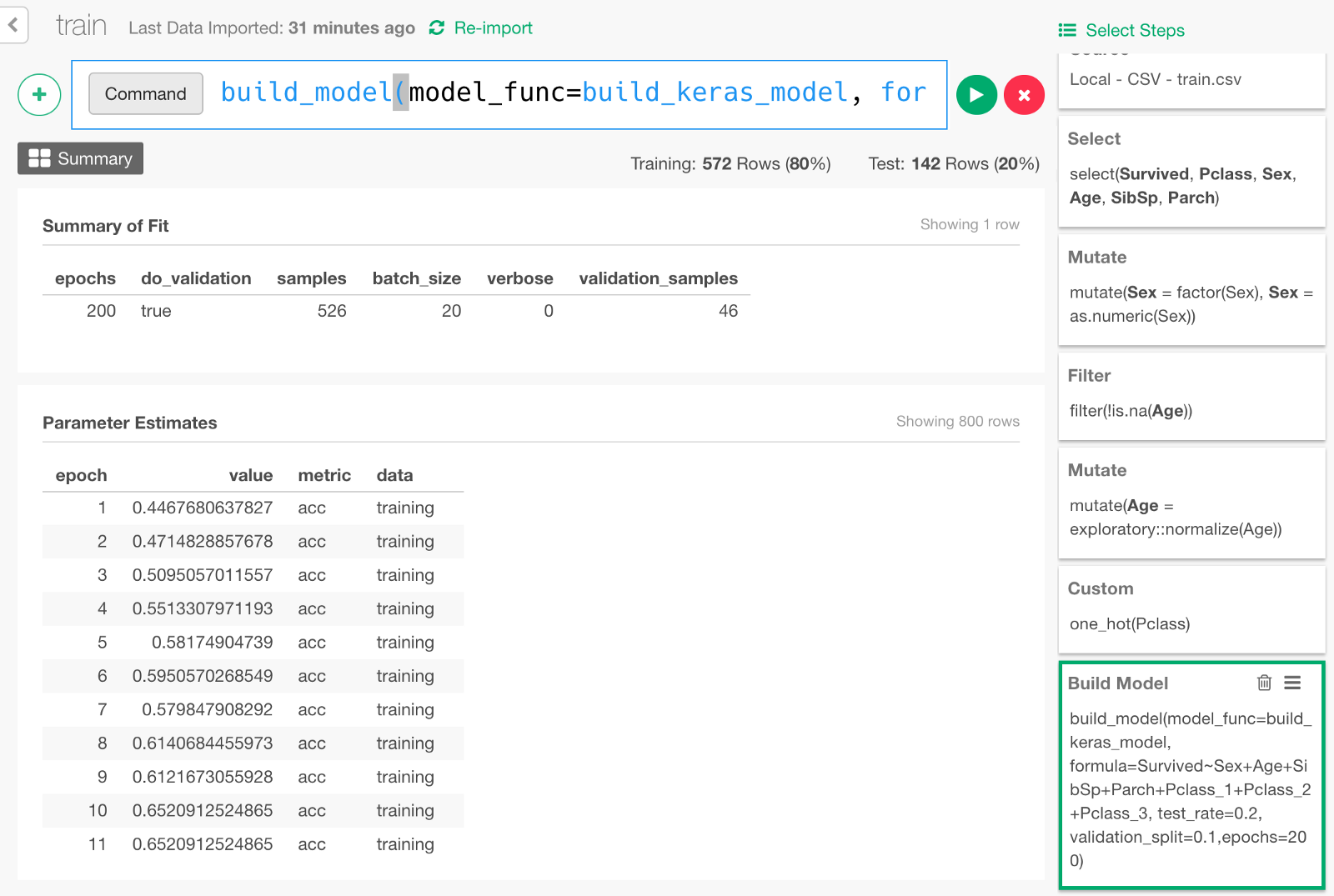
Now the data is ready, finally we are going to build a Deep Learning model by typing the following command.

build_model(model_func=build_keras_model, formula=Survived~Sex+Age+SibSp+Parch+Pclass_1+Pclass_2+Pclass_3, test_rate=0.2, validation_split=0.1,epochs=200)

formula=... means that we are predicting Survived variable with input variables such as Sex, Age, and other columns specified here.

test_rate=0.2 means we keep 20% of the data for testing the prediction performance of the model later.

validation_split=0.1 means we keep 10% of the data for validation (set of tests done in the middle of training to monitor how the model is improving).

Once the model is built, it would look something like below.

Extracting Training Progress Data and Visualizing It

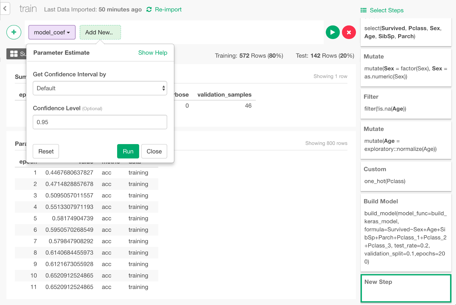
Keras takes the validation data that we discussed earlier and records how the model performed after each round of training as the training goes. We can visualize the model learning performance. From the + button menu, select “Extract Parameter Estimate” menu.

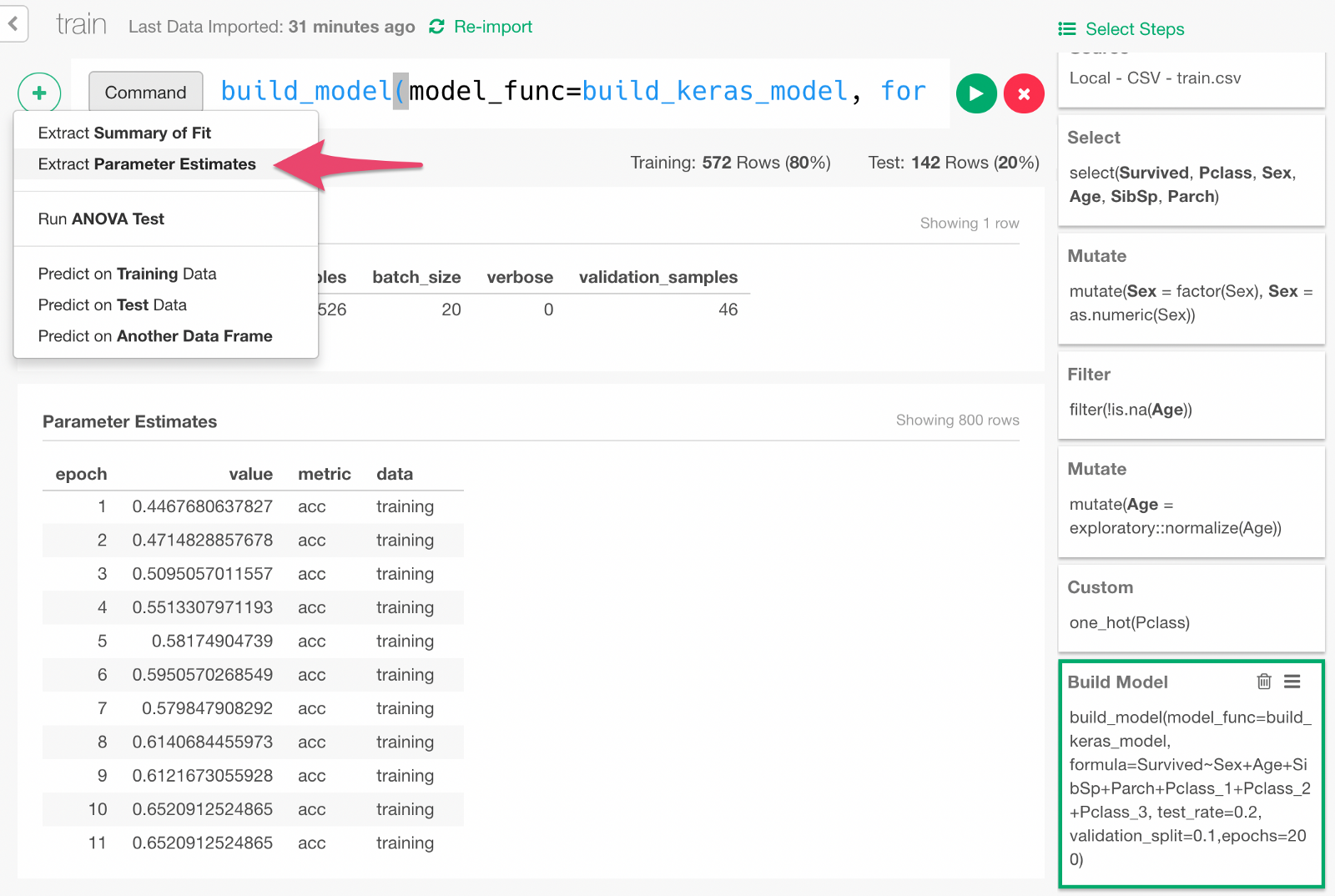
Click Run in the dialog.

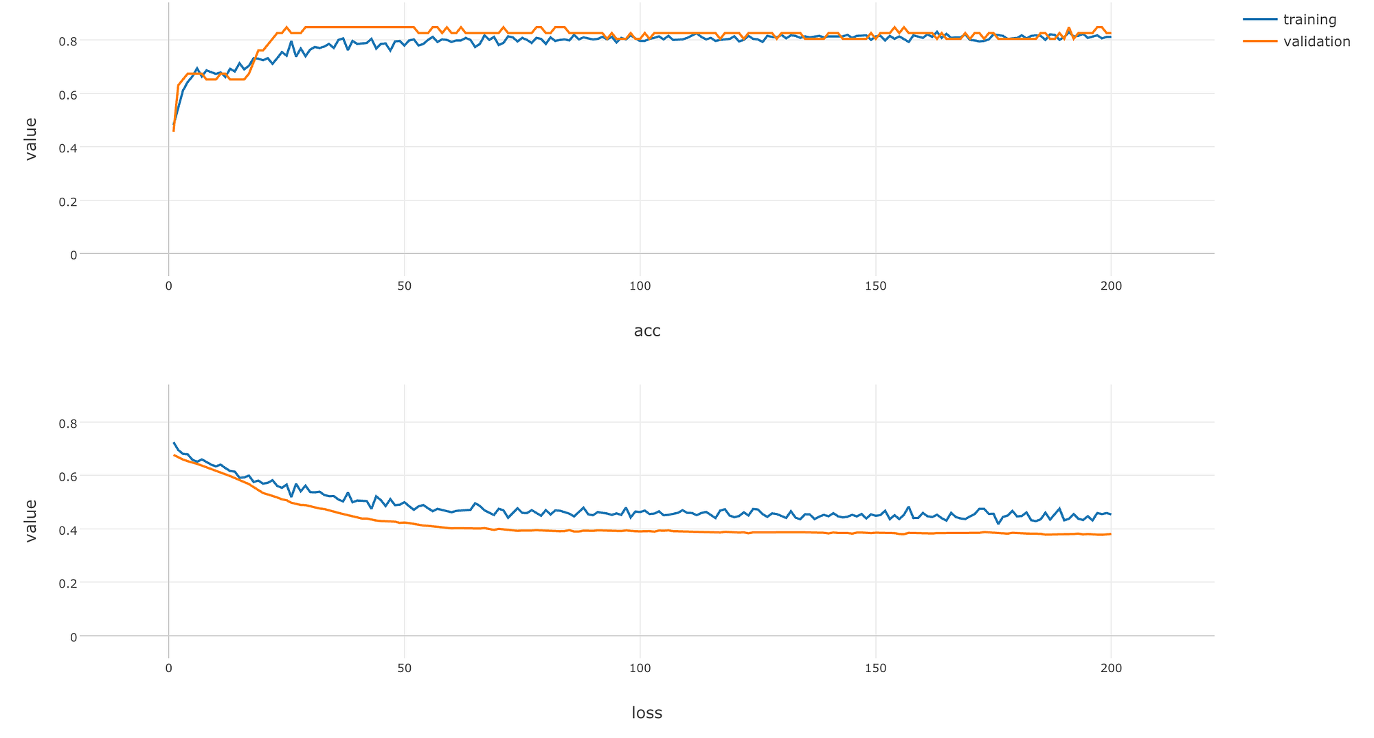
It would looks something like below.

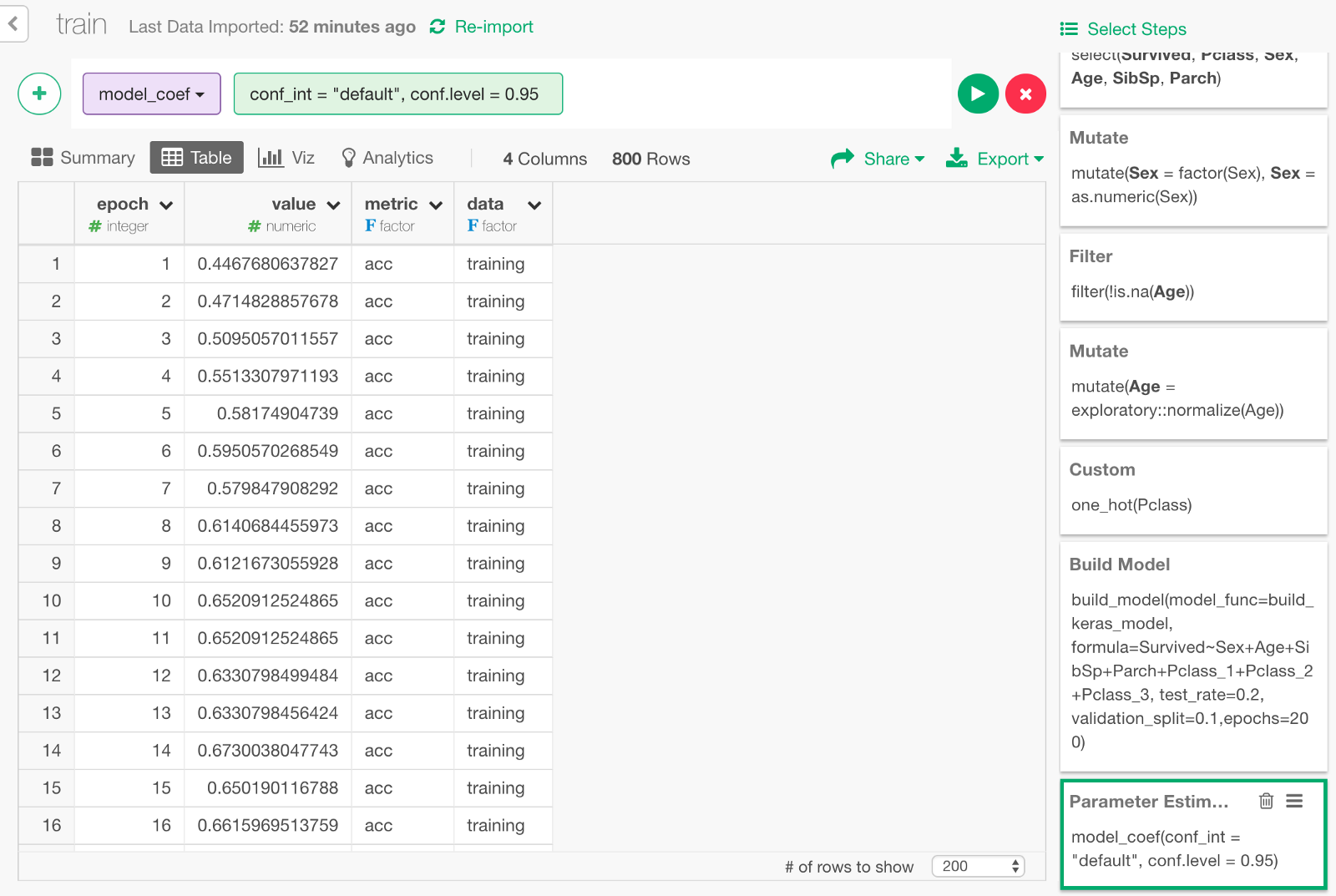
It contains data on how the accuracy (the higher the value is, the smarter the model is) and the loss (the lower the value is, the better the model is) has changed during the training.

• epoch : Number of times rounds of learning were repeated.
• value : The value of accuracy or loss.
• data : Whether a value is based on the validation data or the training data.
• metric : Whether the value of the row is accuracy or loss.

Let’s visualize the data with a line chart like the following.

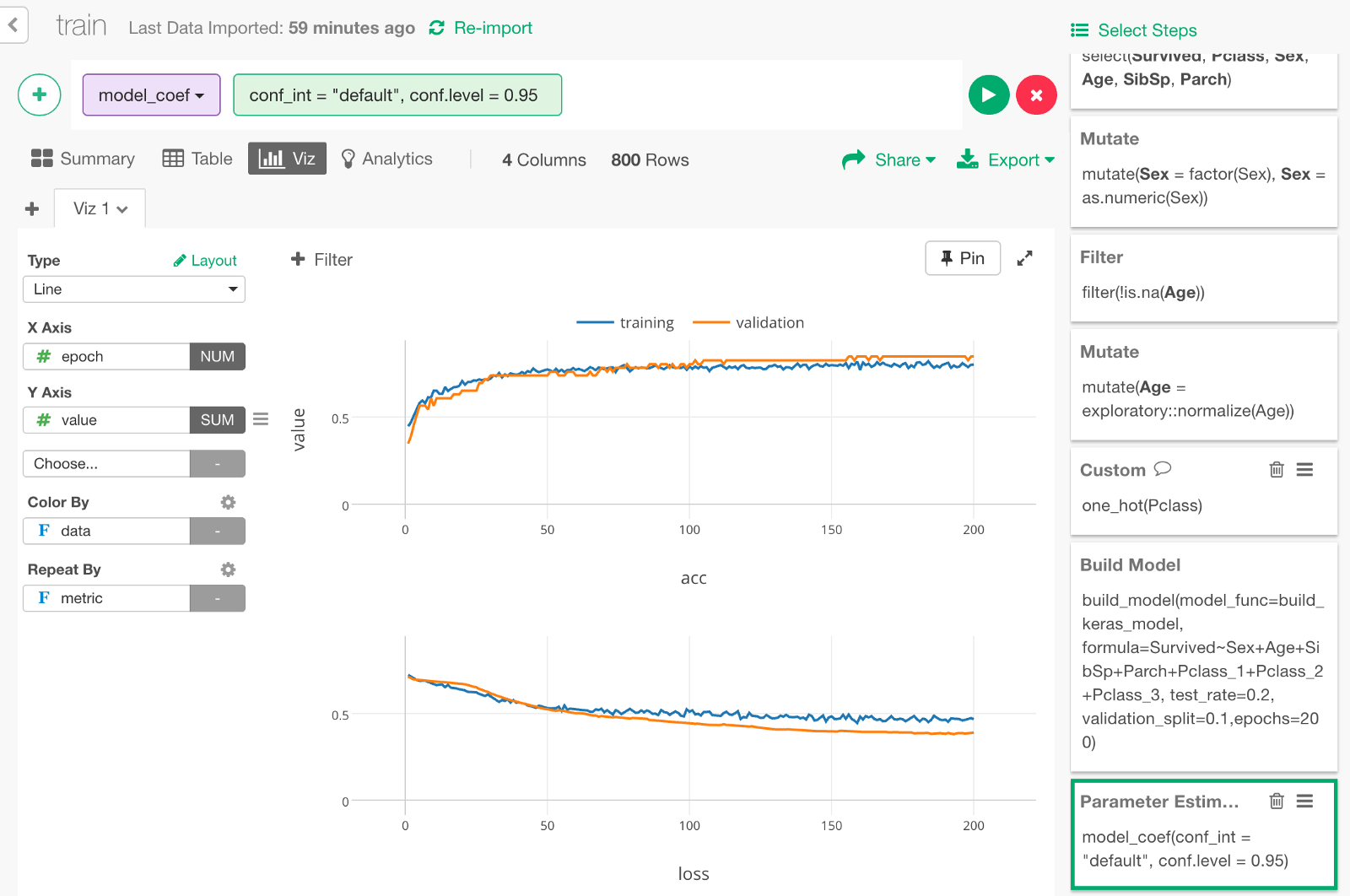
Let’s make the chart full screen and take a look.

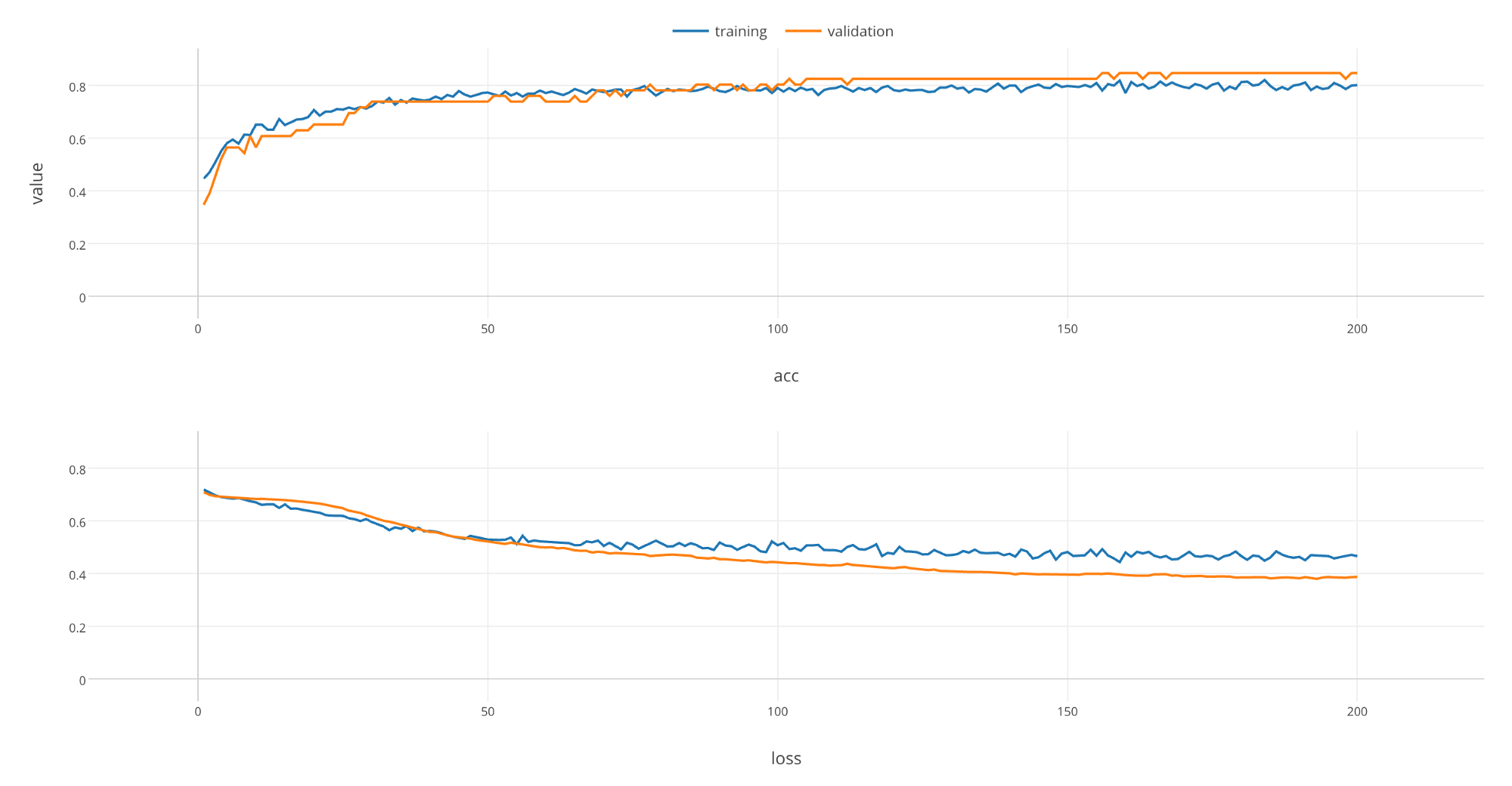
As rounds of learning is repeated, we can see that loss is getting smaller and accuracy is getting larger with both training and validation data. We can see that these changes saturate at the end of learning, which implies that you would not see much improvements on the model even if you repeat rounds of learning any further.

Prediction with the Test Data

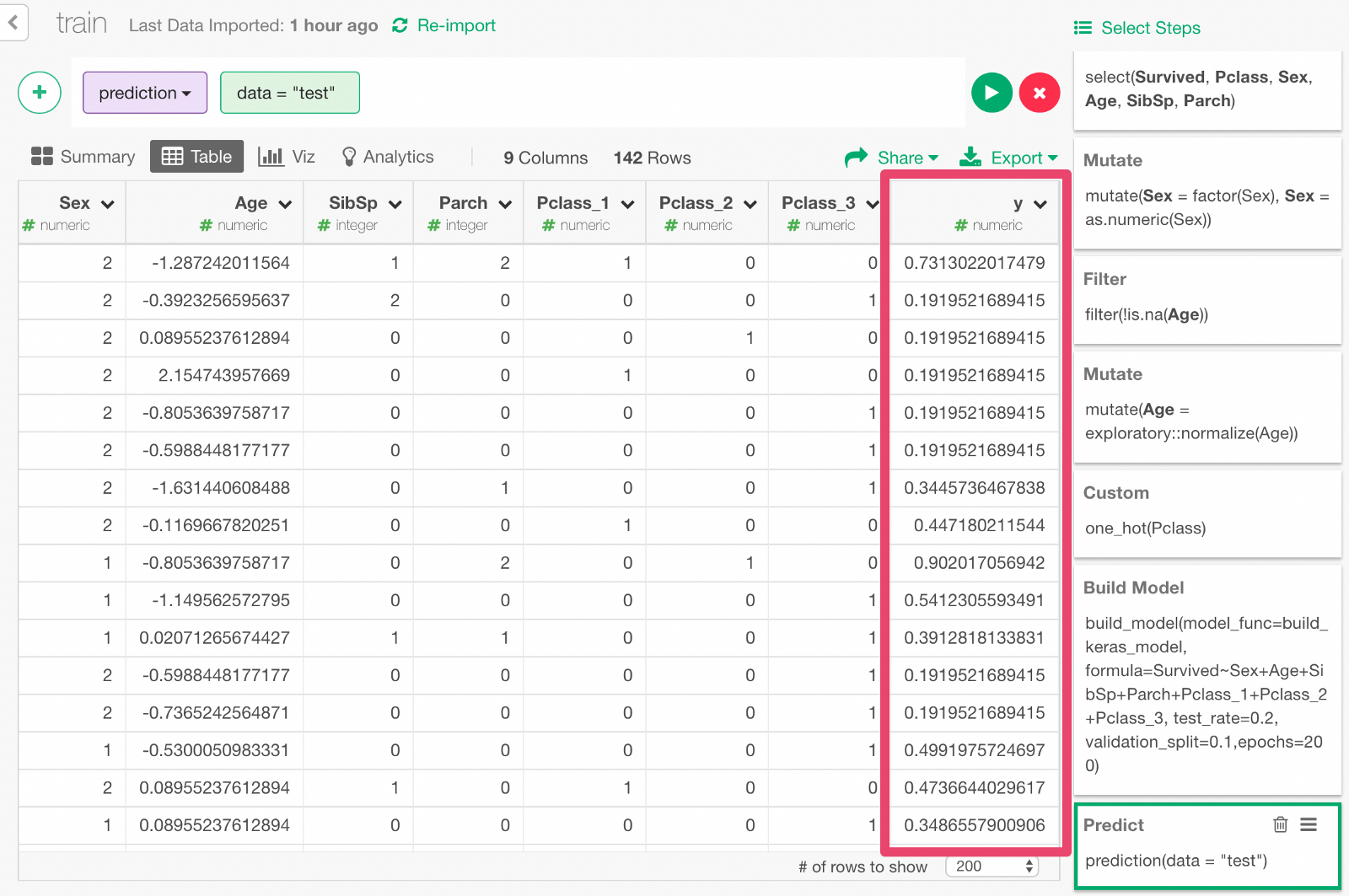
20% of the data is kept as Test data so that we can use this data to predict whether each passenger would survive or not and evaluate the prediction performance.

Click + button and select “Predict on Test Data” menu. In the dialog that comes up, click Run.

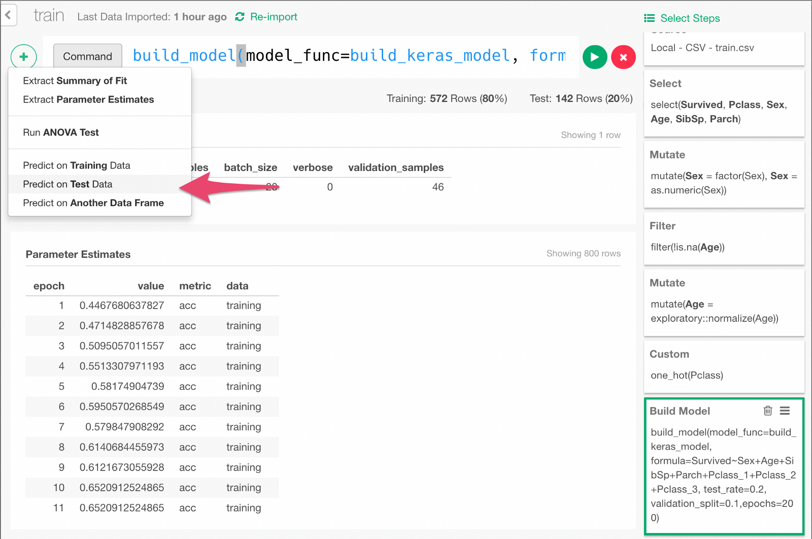
You can see that the y column contains the probability of survival predicted by the model.

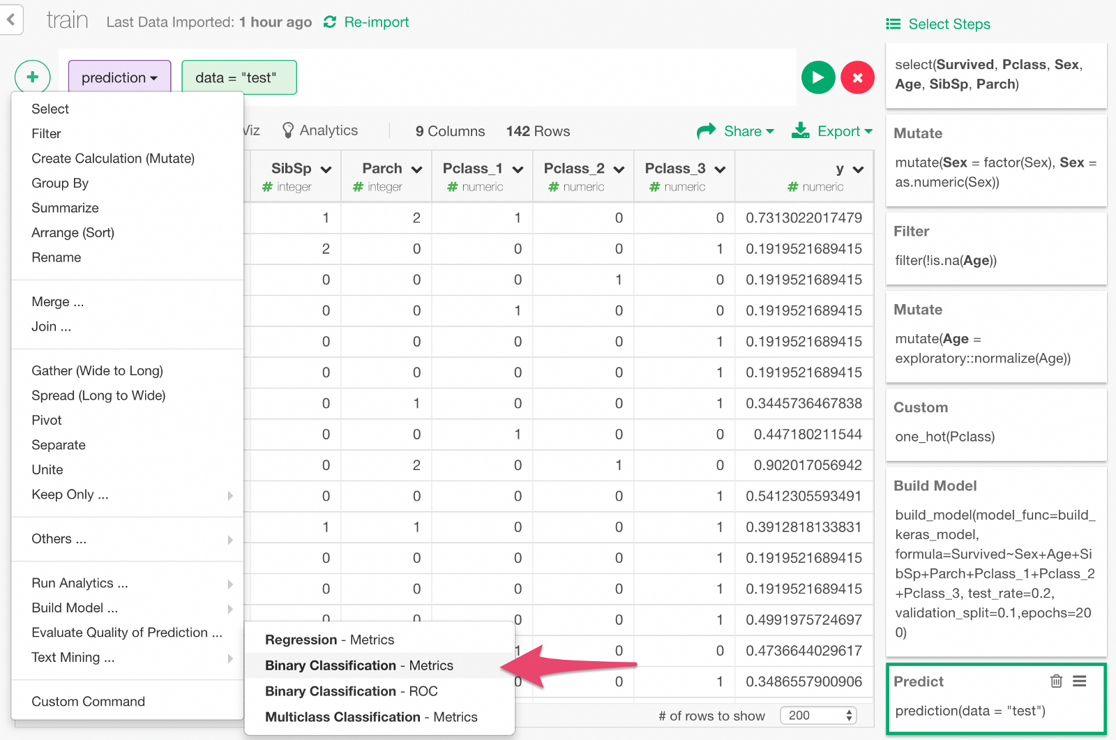
Evaluate accuracy of prediction

Now, we can evaluate the prediction result. From the + menu, select “Binomial Classification —Metrics”.

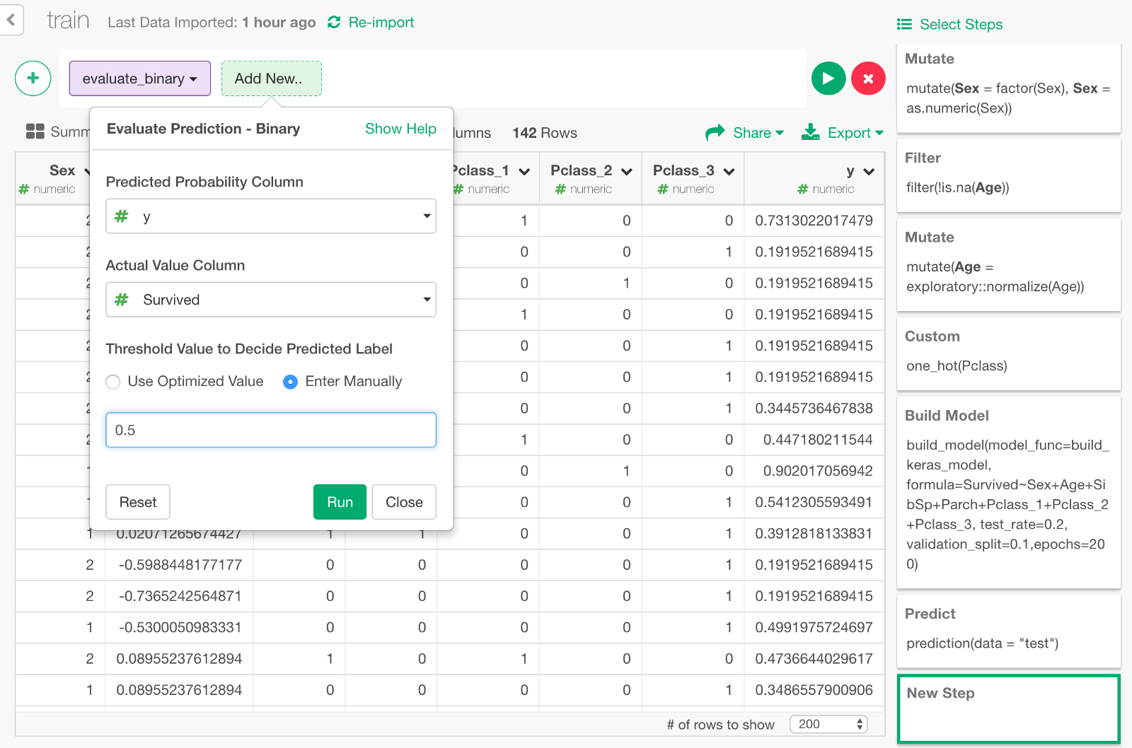
In the dialog, specify the values as follows, to compare the predicted survival probability y and the actual survival result Survive to evaluate the prediction.

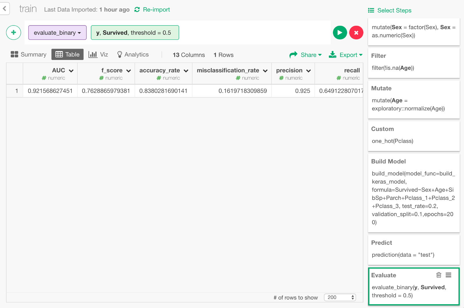
Click Run, and you will see the evaluation result like below. You can see some metrics like Accuracy Rate, AUC, etc.

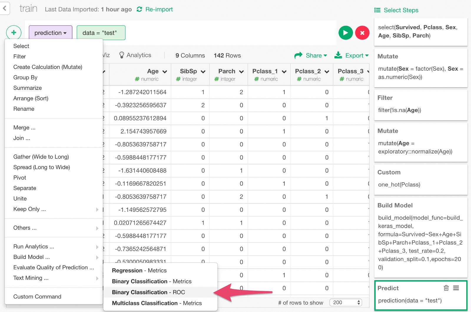
We can also visualize ROC curve, which is a curve that comes up in the process of calculating the AUC. Go back one step before and choose “Binary classification — ROC” from the + button menu.

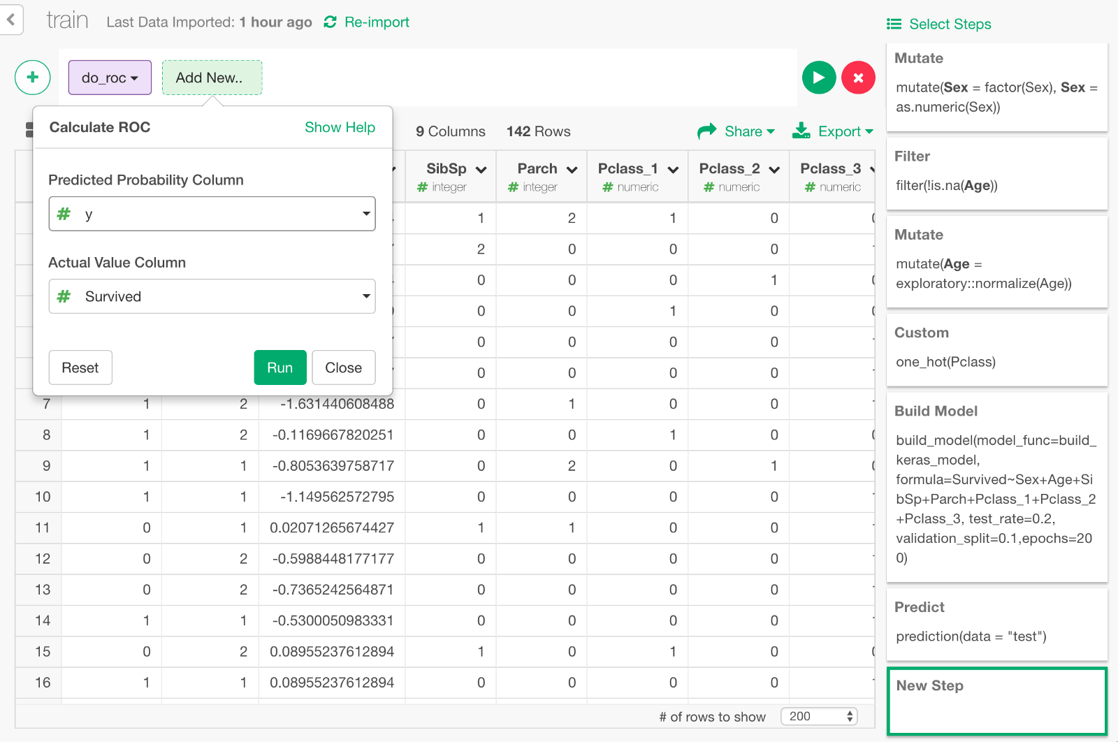
In the dialog, select y and Survived to calculate the ROC curve by comparing those columns.

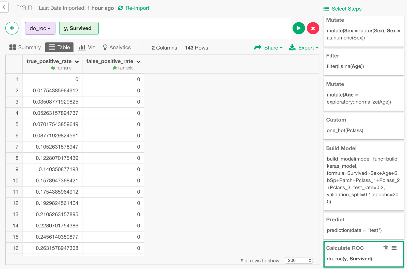
The data for ROC curve is calculated.

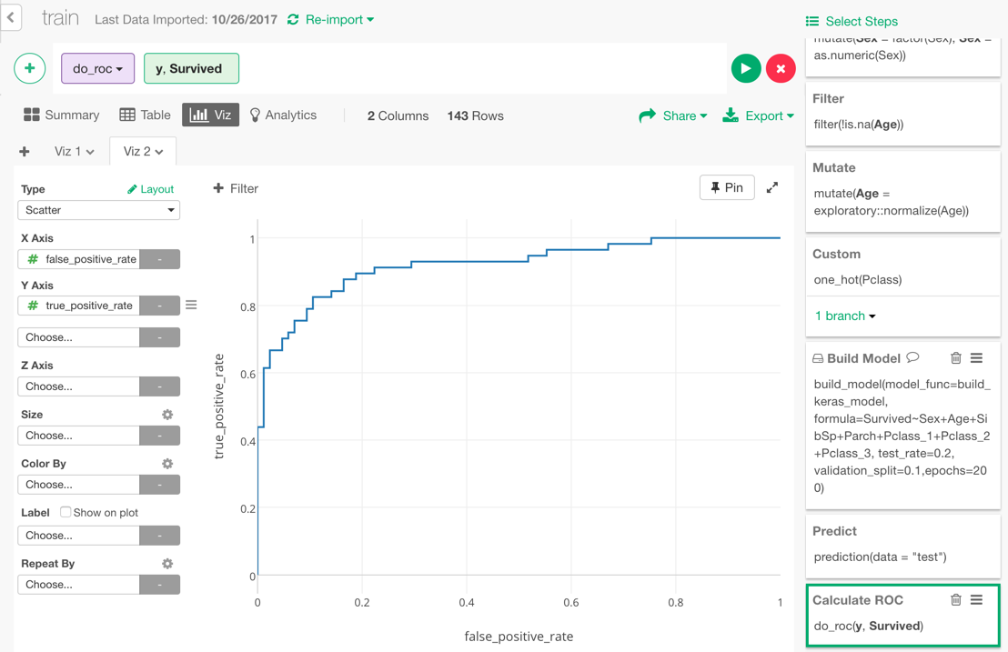
If you visualize the result with Area Chart, it looks like this. The area of the blue part under the curve is 0.92, which is the value of AUC we got earlier.

By the way, ROC curve is useful especially when you want to compare multiple models prediction performance. For example, here I’m comparing this model by Keras and another model by Random Forest.

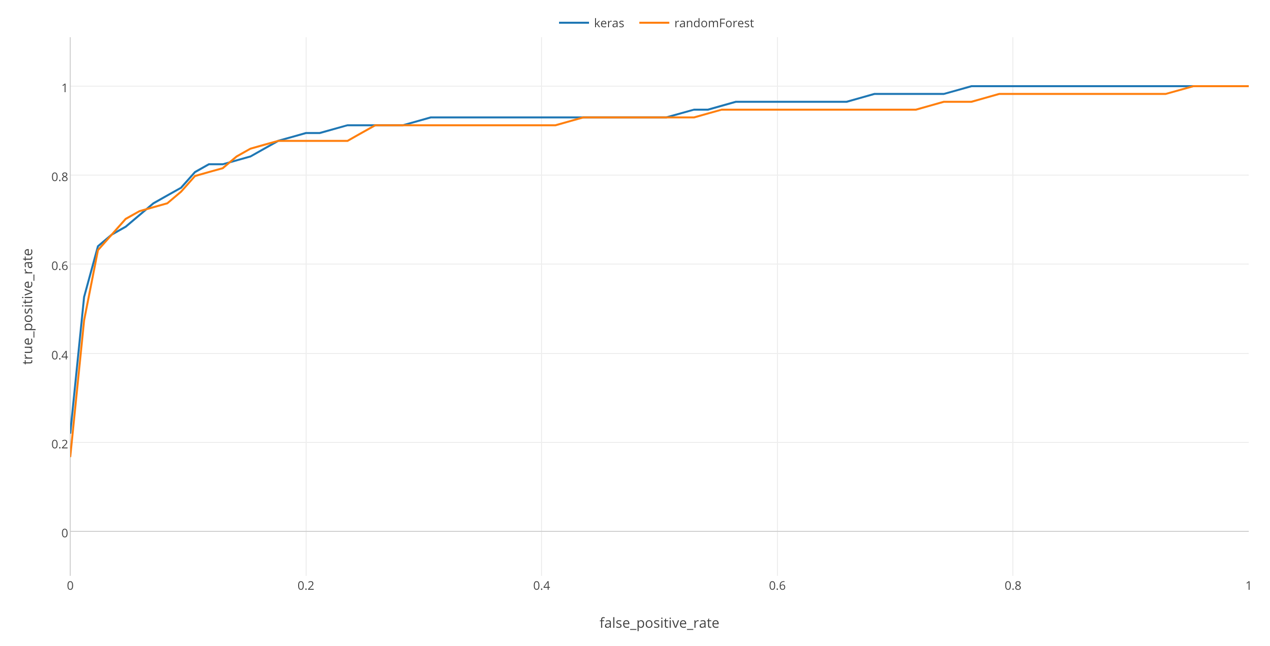
In this chart, we can see that Keras has a slightly larger area than Random Forest, which means that it was able to separate those who survived from those who did not more clearly, in this data. (However, this can be affected by chances. When I tried several times, there were times when randomForest performed better than Keras.)

Adjusting Neural Network

If you would like to further adjust the Deep Learning model, try changing the following part of the script. When you press the Save button after changing it, the function is updated in R. As it is in this script, Neural Network with three layers with 7, 5, and 1 neuron in respective layers is constructed.

# Create three-layer Neural Network Model
  model <- keras_model_sequential()
  model %>%
    layer_dense(units = 7, activation = 'relu', input_shape = c(7)) %>% # Set 7 nuerons in the first layer
    layer_dropout(rate = 0.2) %>% # dropout 20% of the data
    layer_dense(units = 5, activation = 'relu') %>% # Set 5 neurons in the second layer
    layer_dropout(rate = 0.1) %>% # dropout 10% of the data
    layer_dense(units = 1, activation = 'sigmoid') # Summarize them as a one survival probability in the third layer

Summary

We have just predicted the survival of the Titanic passengers with a Deep Learning model via Keras. The number of passengers in the Titanic data is only about 900, and it is clearly not the kind of data where Deep Learning would show its true power. But for this exercise, I picked this data as an interesting and accessible problem to try and get used to Keras.

In my next post, I will write about making use of deep learning for larger data. I’m also planning to write about other favorite models at kaggle, such as Random Forest, XGBoost, etc. Stay tuned!