Using H2O Powered Machine Learning Algorithms in R & Exploratory

H2O is a popular open source machine learning library and is known for its speed and scalability. It is designed to produce a much faster performance compared to other machine learning tools especially as the data becomes bigger. It supports a set of the modern machine learning algorithms including deep learning, ensemble trees such as XGBoost, RandomForest, etc. It provides various interfaces including R and Python so that the users of those languages can easily access the power of H2O. Today, I’ll demonstrate how to use H2O library in Exploratory, which is known as an UI for R.
I have US flight delay data that is about one million rows. And I’ll use RamdomForest algorithm from H2O to build a model to predict whether a given flight will be late at the departure time.
Setup
Installing and starting H2O
Download H2O from their download page, and start H2O process from shell, like below.
    cd ~/Downloads
    unzip h2o-3.14.0.3.zip
    cd h2o-3.14.0.3
    # Start with 8GB of memory
    java -Xmx8g -jar h2o.jar
Installing R package “h2o”
The h2o R package on CRAN lags a little behind, and it does not connect to the latest-stable version we just downloaded.
So we want to download the latest R package directly from H2O’s server, then we can install it inside Exploratory. Also, there are two R packages that are pre-requisite for H2O. They’re statmod and RCurl, which we can install inside Exploratory as well.
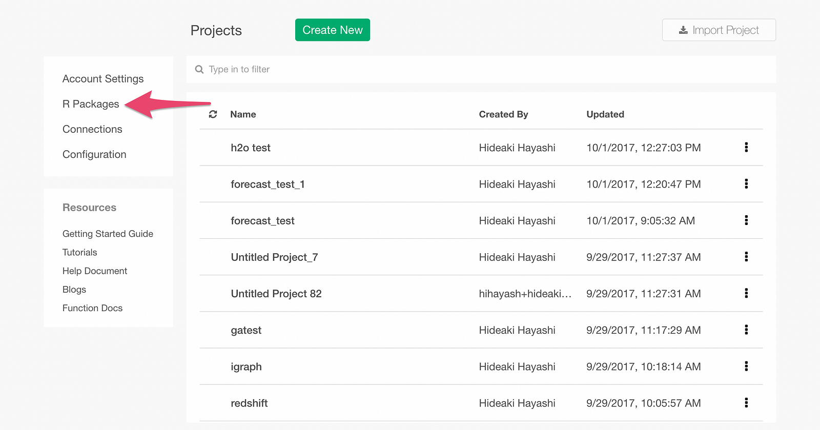
From Exploratory’s Project List page, click R Package menu.
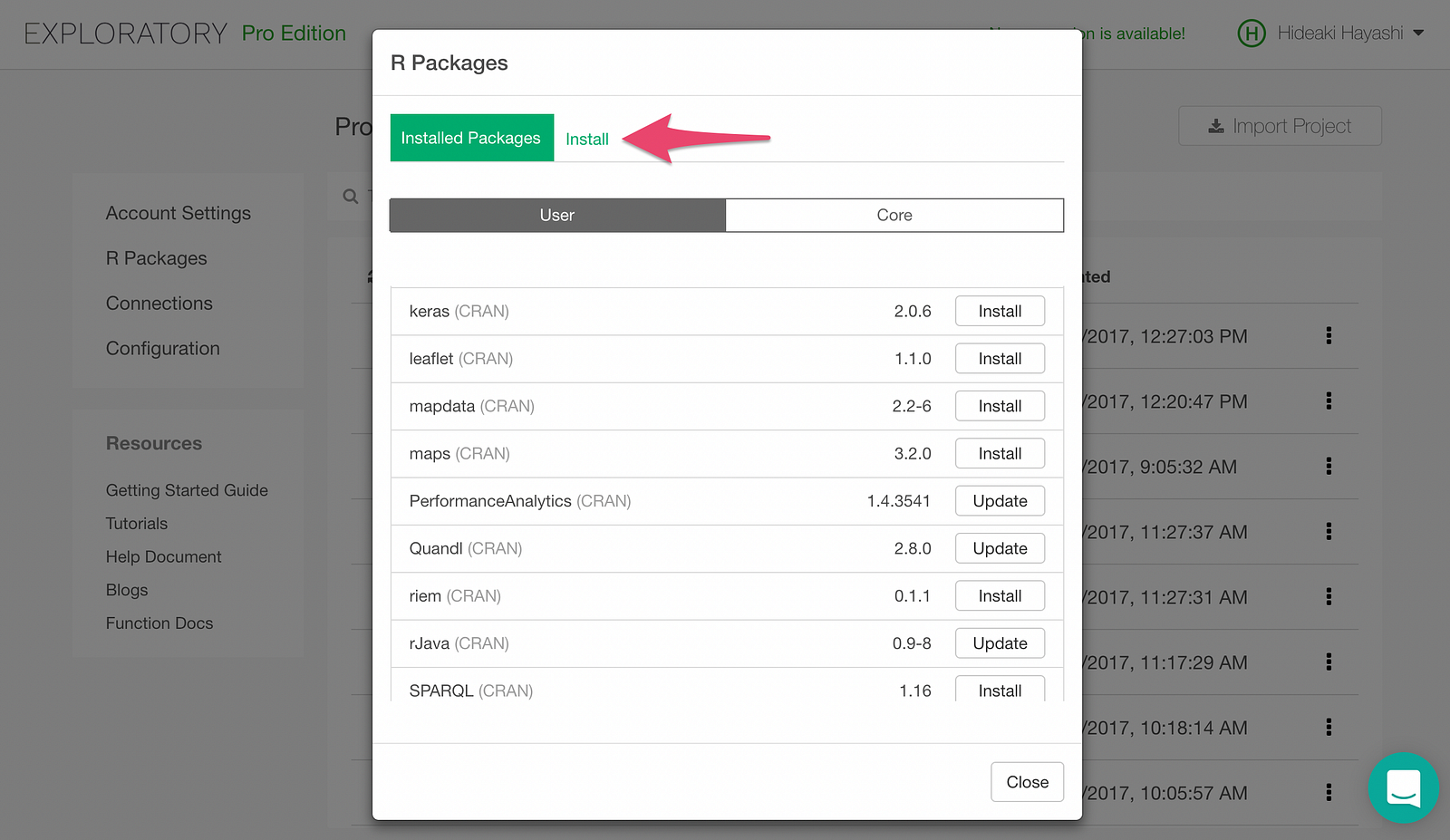
Click Install tab.
Type in “statmod” and click Install button. statmod will be installed.
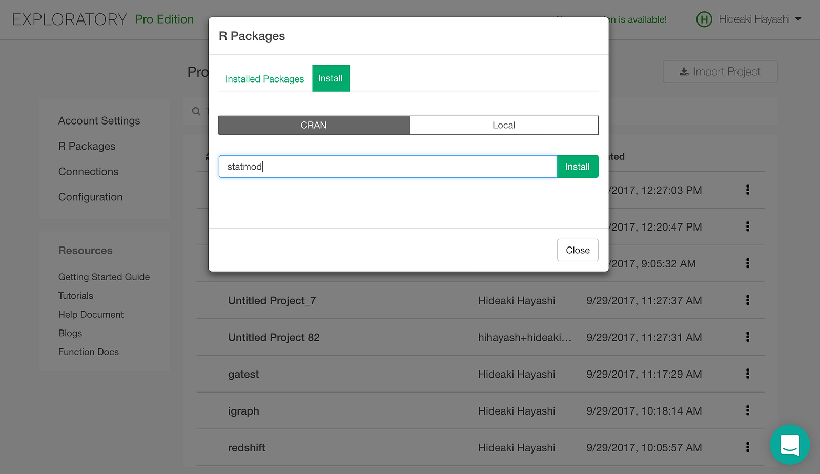
Install RCurl the same way.
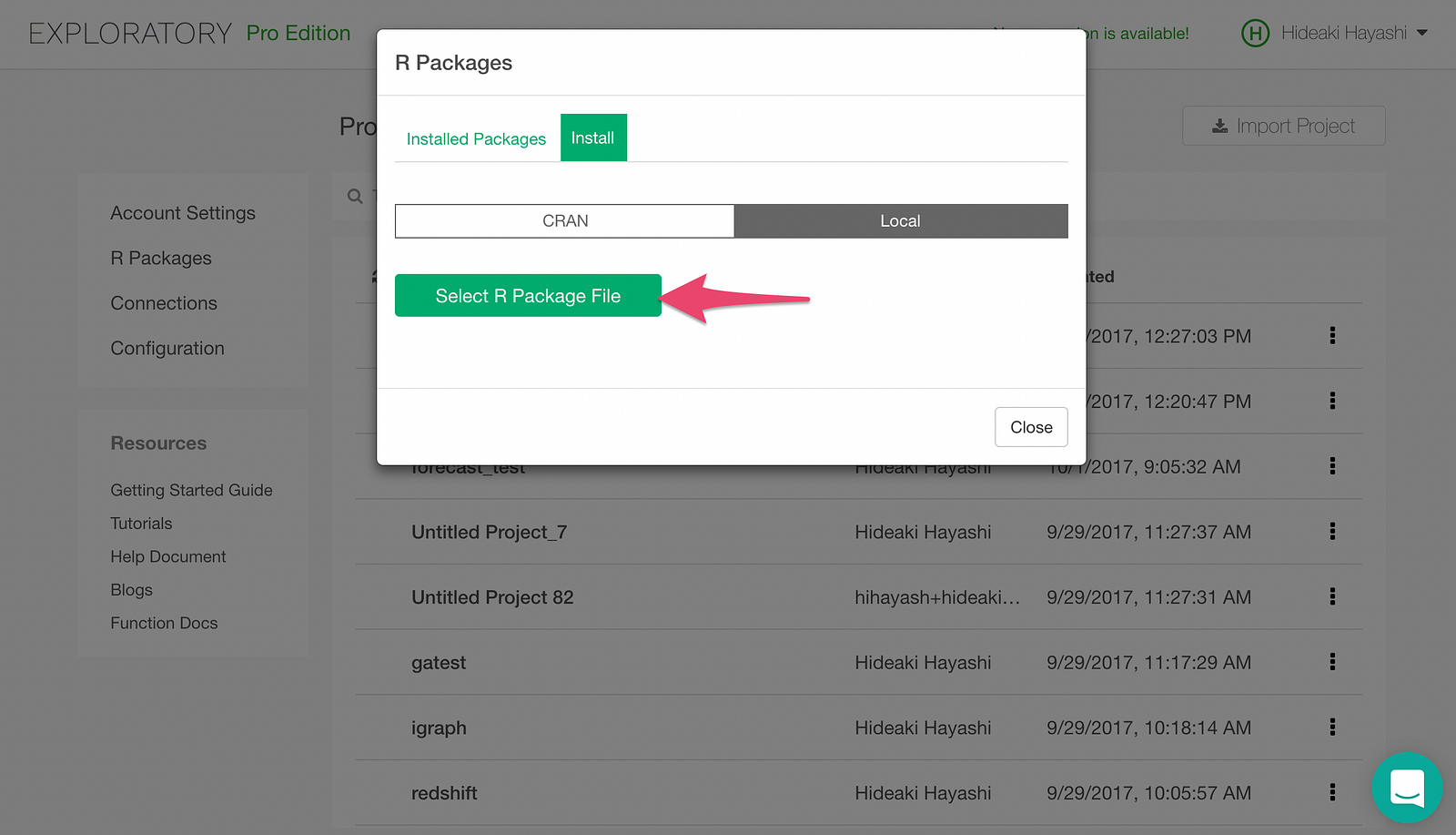
Now, let’s install h2o package, which we download from here. Click Local Install tab.
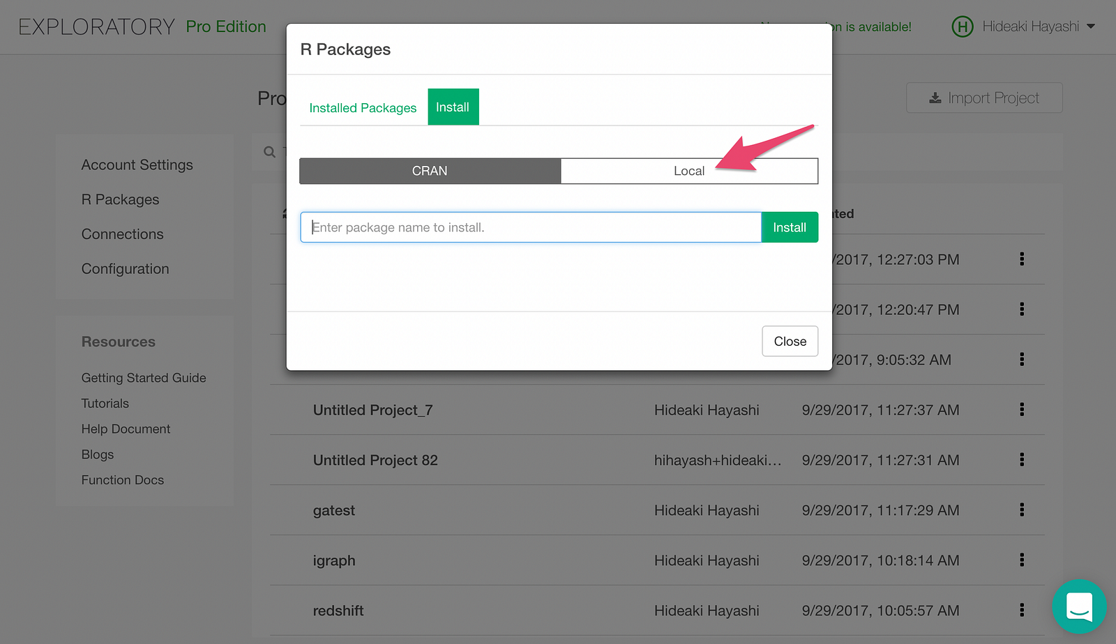
Clicking “Select R Package File” button will pop up a file picker. Pick the h2o_3.14.0.3.tar.gz file we downloaded earlier, and h2o package will be installed.
Register H2O RandomForest as a Custom Model in Exploratory
Exploratory supports many machine learning algorithms through a simple UI experience out of the box. Also it provides a model extension framework with which you can flexibly add your custom models by writing custom R scripts.
If you want to know more details on how to use the model extension framework please take a look at this document page.
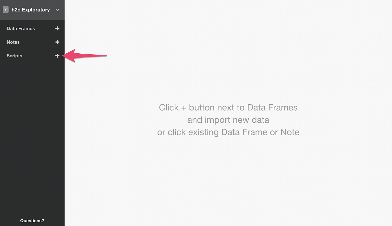
Let’s create a Custom Script in an Exploratory Project, by clicking + icon for Scripts menu.
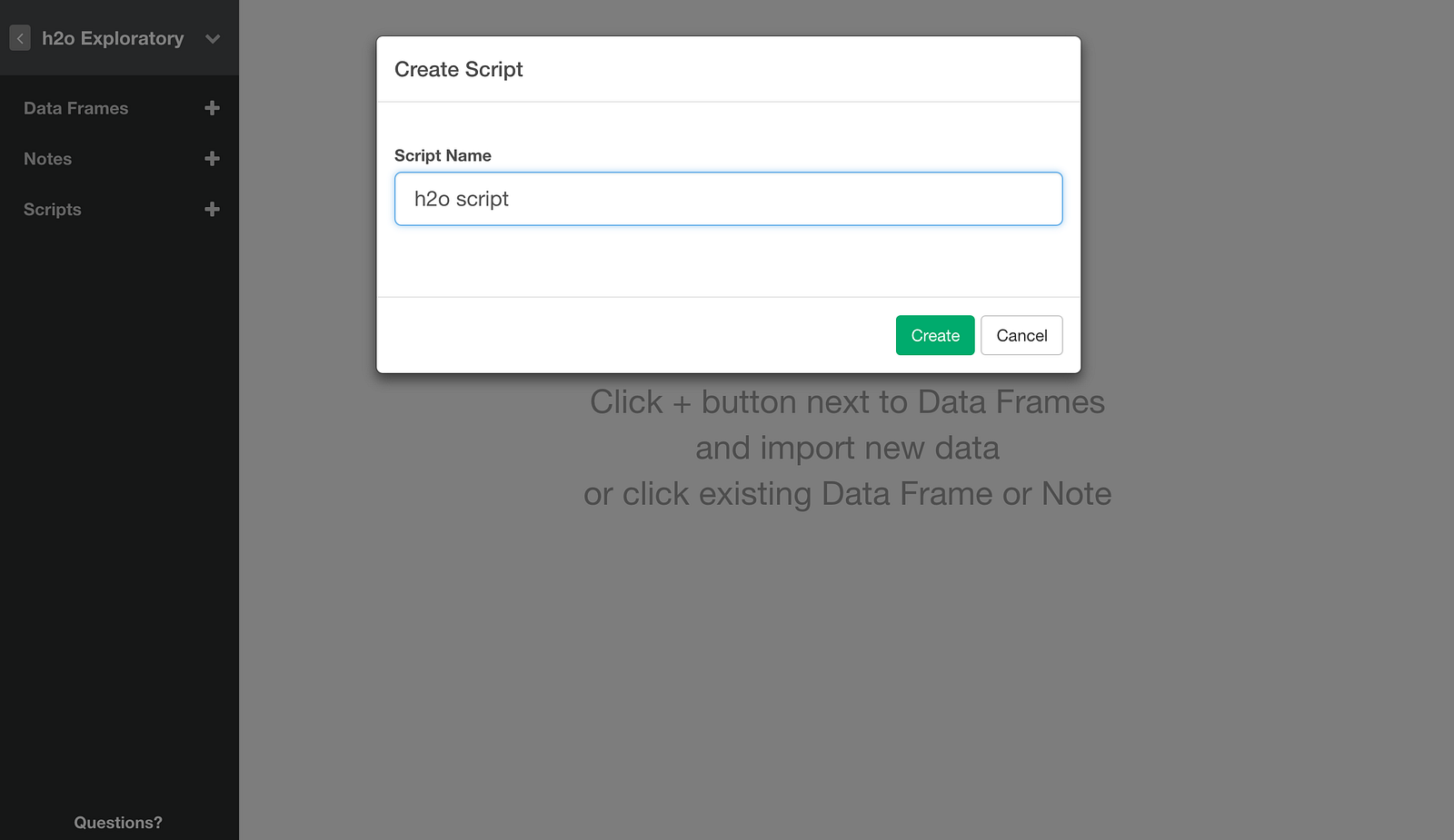
Then type in a name for the script, and click Create button.
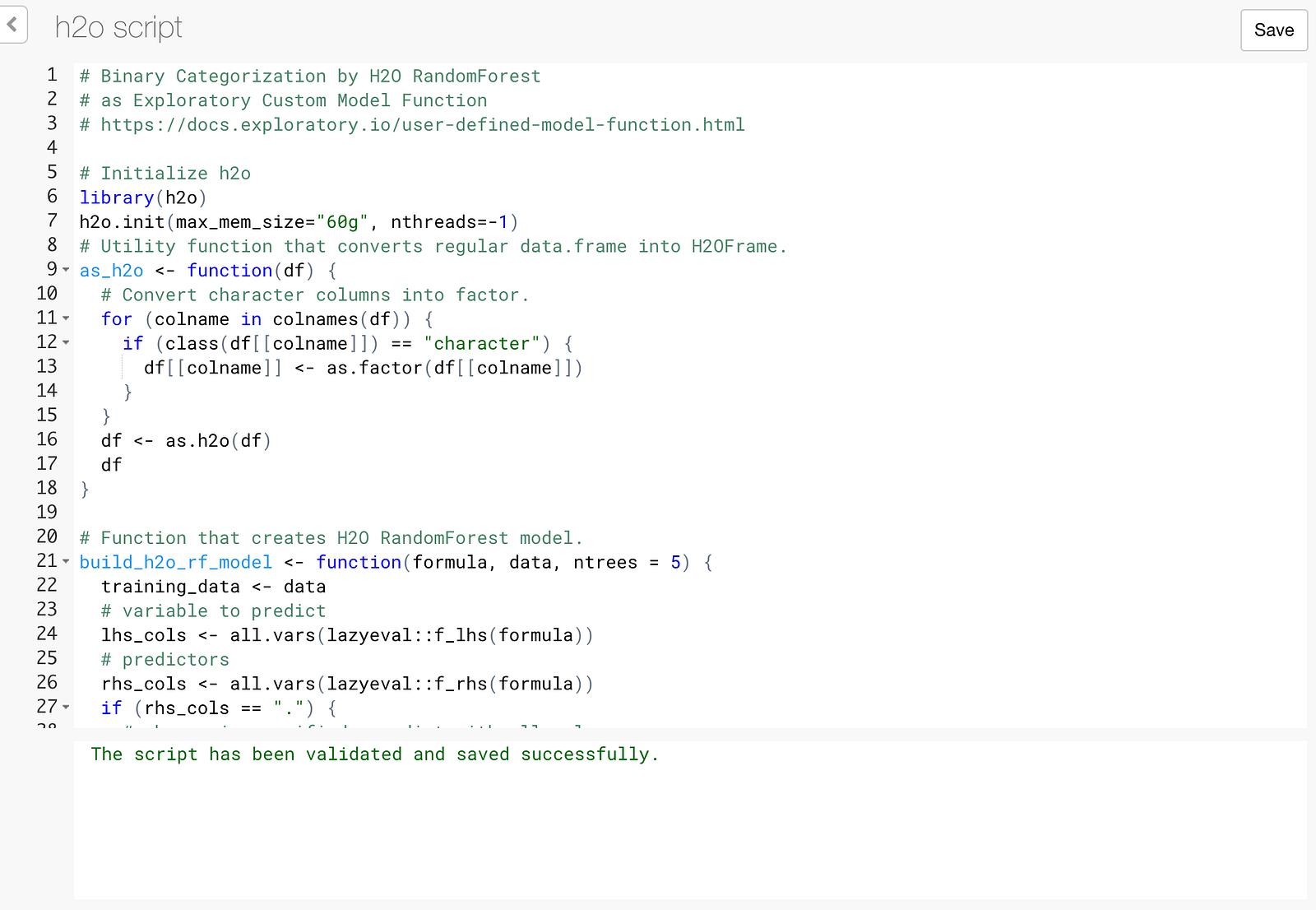
Script editor will open up.
Here is R script that makes use of the framework to make H2O RandomForest available from Exploratory.
# Binary Categorization by H2O RandomForest
# as Exploratory Custom Model Function
# https://docs.exploratory.io/user-defined-model-function.html
# Initialize h2o
library(h2o)
h2o.init(max_mem_size="60g", nthreads=-1)
# Utility function that converts regular data.frame into H2OFrame.
as_h2o <- function(df) {
  # Convert character columns into factor.
  for (colname in colnames(df)) {
    if (class(df[[colname]]) == "character") {
      df[[colname]] <- as.factor(df[[colname]])
    }
  }
  df <- as.h2o(df)
  df
}
# Function that creates H2O RandomForest model.
build_h2o_rf_model <- function(formula, data, ntrees = 5) {
  training_data <- data
  # variable to predict
  lhs_cols <- all.vars(lazyeval::f_lhs(formula))
  # predictors
  rhs_cols <- all.vars(lazyeval::f_rhs(formula))
  if (rhs_cols == ".") {
    # when . is specified, predict with all columns.
    rhs_cols <- colnames(training_data)[colnames(training_data) != lhs_cols]
  }
# convert training data into H2OFrame.
  training_data <- as_h2o(training_data)
  # Train RandomForest model with H2O.
  md <- h2o.randomForest(x = rhs_cols, y = lhs_cols, training_frame = training_data, ntrees = ntrees)
  # Return model and formula as one object.
  ret <- list(model = md, formula = formula)
  class(ret) <- c("h2o_rf_model")
  ret
}
# function to predict on new data with the trained model
augment.h2o_rf_model <- function(x, data = NULL, newdata = NULL, ...) {
  if (is.null(data)) {
    data <- newdata
  }
  formula <- x$formula
  h2o_data <- as_h2o(data) # convert data into H2OFrame.
  # predict with the model.
  predicted_data <- h2o.predict(x$model, h2o_data)
  # convert predicted data back to data.frame.
  predicted_data <- as.data.frame(predicted_data)
  # bind the predicted data with original data, and return it
  ret <- bind_cols(data, predicted_data)
  ret
}
# Return model's predictive performance metrics so that
# they are displayed in "Summary of Fit" table
# in model summary view.
glance.h2o_rf_model <- function(x, ...){
  mdperf<-h2o.performance(x$model)
  h2o.metric(mdperf)
}
# Return variable importance so that
# they are displayed in "Parameter Estimates" table
# in model summary view.
tidy.h2o_rf_model <- function(x, ...){
  h2o.varimp(x$model)
}
Copy the above script into the script editor.
While H2O process is up and running, click Save button.
Now we are ready to use H2O’s RandomForest algorithm through Exploratory’s UI. Let’s try it!
Getting the Data Ready
Download the data
Here is a cool github repository by Szilard Pafka, with benchmark that compares various predictive platforms.
I’m borrowing the data he compiled for his benchmark from the famous flight delay data. You can download the data with 1 million flights I’m using in this exercise from here.
Import the downloaded CSV Data into Exploratory
Unzip the downloaded file and import into Exploratory.
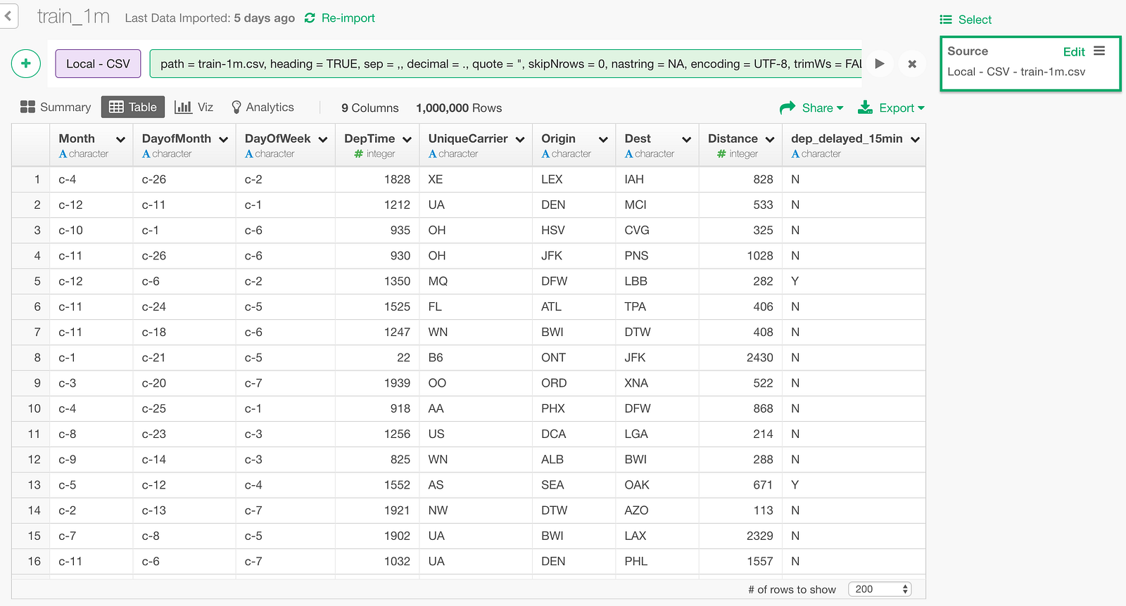
One row in this data represents one flight. There are following 9 columns.
- Month : Month of the flight
- DayofMonth : Day of the month of the flight
- DayOfWeek : Day of the week of the flight
- DepTime : Departure time
- UniqueCarrier : Airline Carrier Code
- Origin : Originating airport code
- Dest : Destination airport code
- Distance : distance between origin and destination
- dep_delayed_15min : whether the departure of the flight was late for more than 15 minutes
Build a RandomForest model
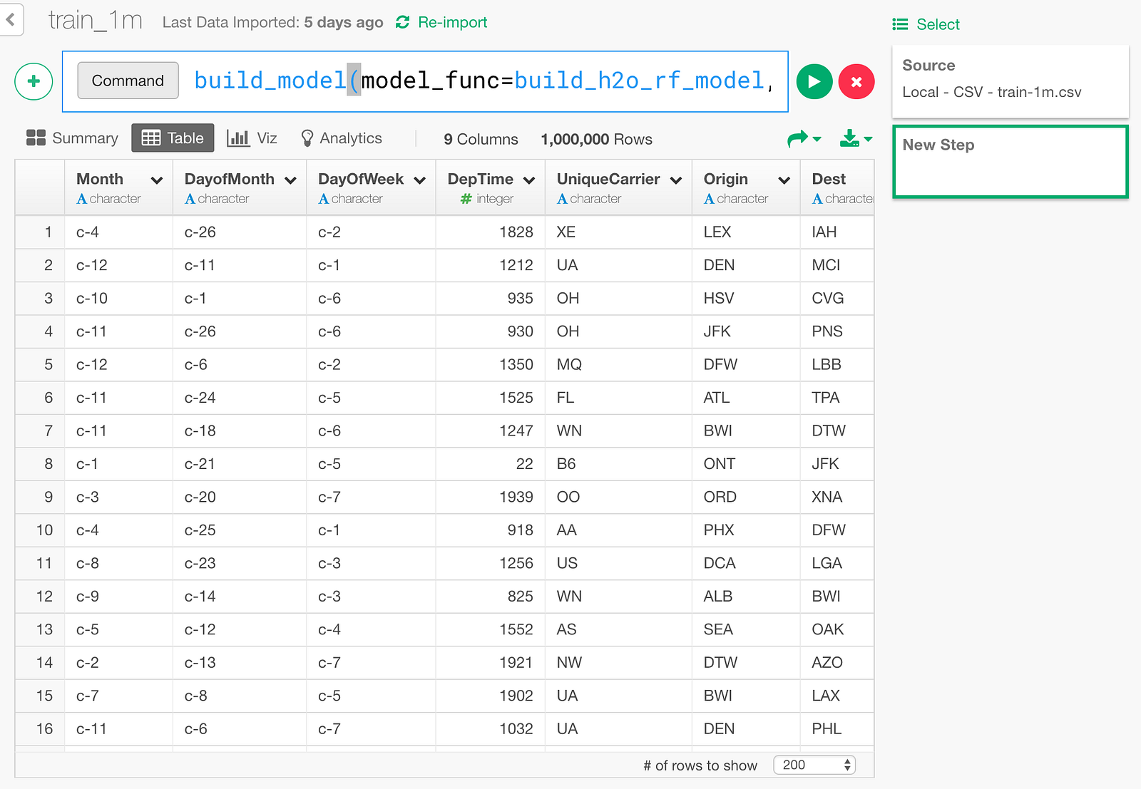
Let’s build a RandomForest model that predicts the dep_delayed_15min column which shows whether flights delayed more than 15 minutes, based on
all the other columns.
Type in the following command like below.
build_model(model_func=build_h2o_rf_model, formula=dep_delayed_15min~., test_rate=0.01, ntrees=50)test_rate=0.01 here means keeping 1% of the data for test, without using for training.
Click the “Run” button.
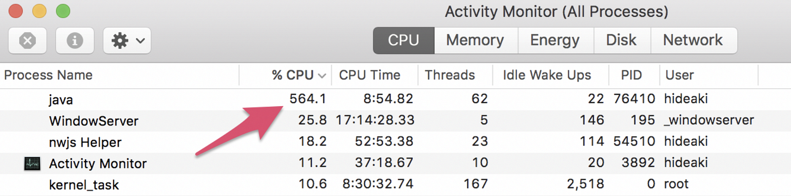
On my MacBook Pro (2016), the training finishes in 2 minutes and a little more. If I open Activity Monitor meanwhile, I see the java process on which H2O is running at the top of the CPU consumption list.
564% would mean it is making use of about 5.64 CPU cores in parallel, which would be contributing its reputation on fast performance.
Here is the screen shown when the training is over and model creation is done.
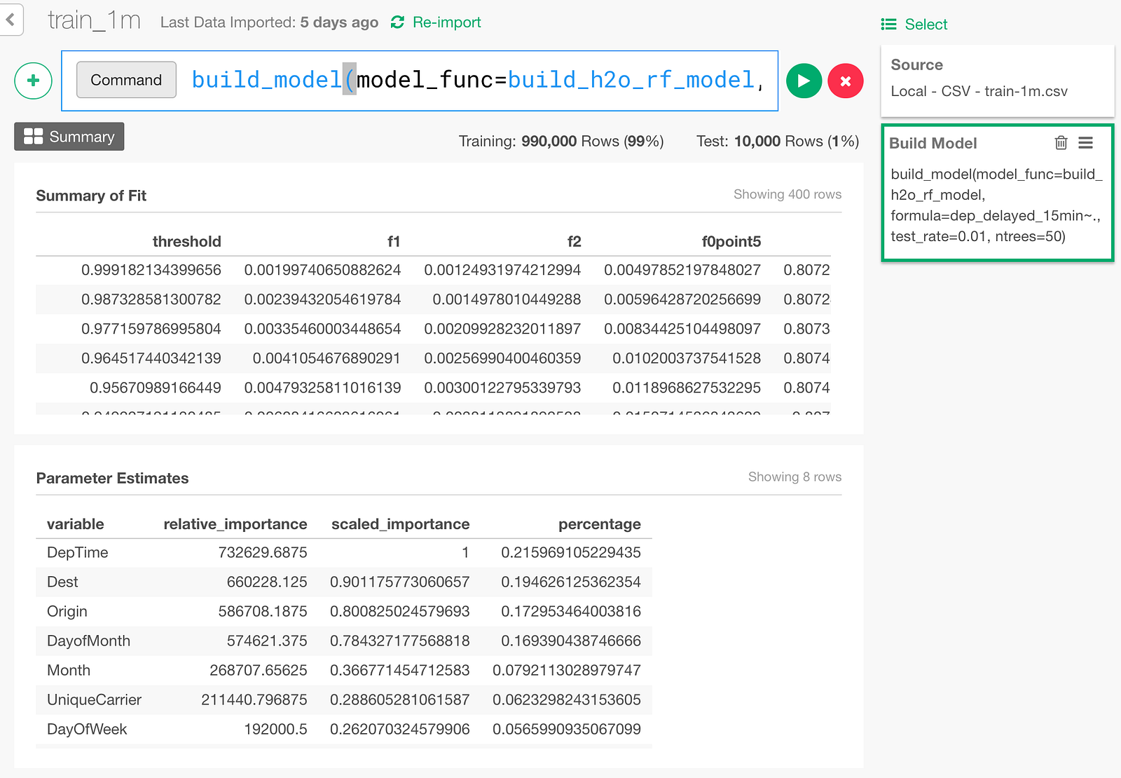
Summary of Fit table shows predictive performance measured with the training data itself, and Parameter Estimates table actually shows Variable Importance.
This Variable Importance is the same thing as we show in “Variable Importance” Analytics View in Exploratory, which is explained with more detail in this document.
Prediction
Remember the 1% data we put aside for test? Let’s predict for the test data by using this model.
Open Prediction dialog from following menu.
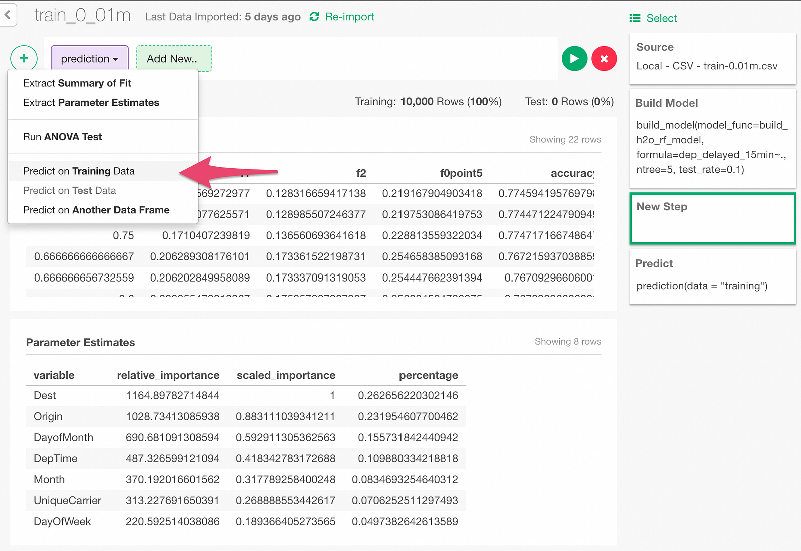
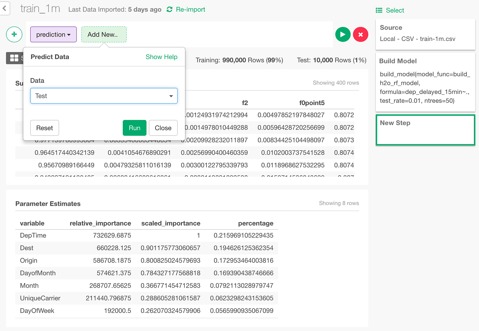
In the Prediction dialog, select ‘Test’ to predict on the test data.
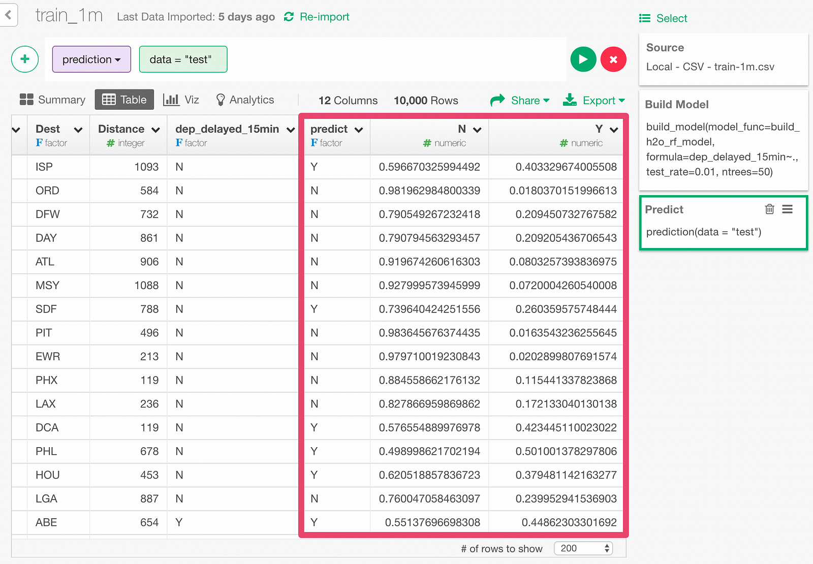
The prediction result appears as below.
Y and N respectively shows the predicted probability of the flight being late more than 15 minutes or not.
Evaluation of predictive quality
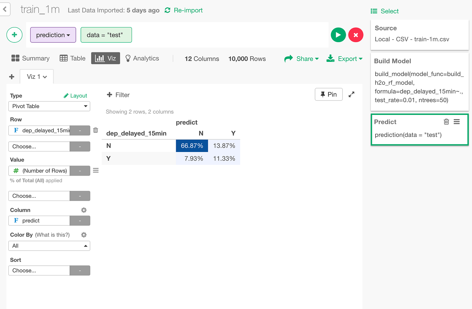
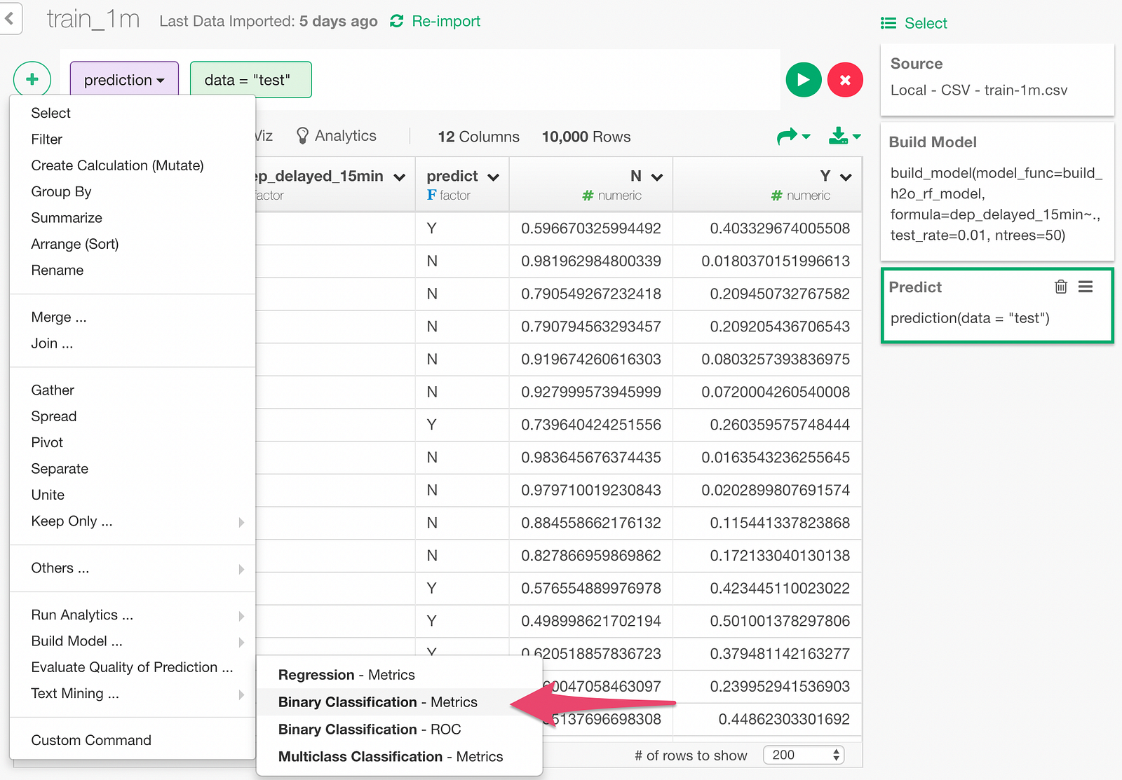
Let’s create a confusion matrix, which is a table that compares the prediction result and actual data, to evaluate the prediction result.
Next, let’s look at the model metrics to evaluate the predictive performance of the model.
Click “Binary Classification — Metrics” menu.
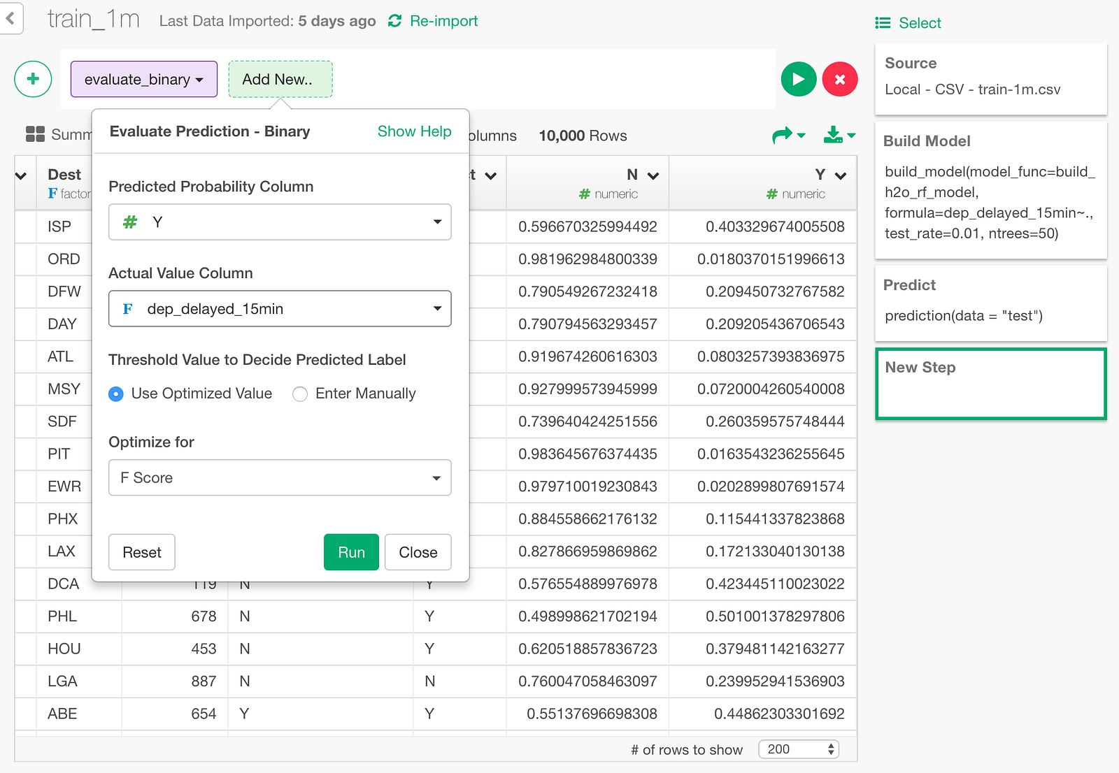
Then, in the dialog, pick the predicted probability column (Y column), and the actual value column (dep_delayed_15min).
Here is the result.
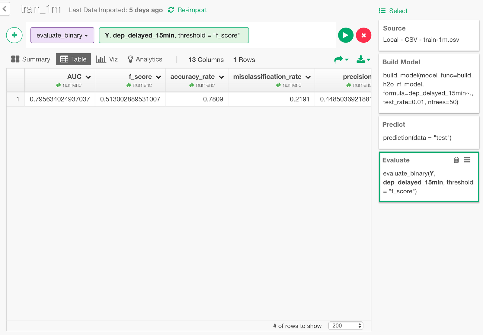
Accuracy rate being 0.7809 means that 78.09% of the time, the predictions were correct.
Also, AUC is an index that shows how cleanly the model’s predicted probability separates the delayed cases and not-delayed cases. It’s a number between 0 and 1, 0.5 meaning no better than random guess. 0.7956 sounds reasonably good.
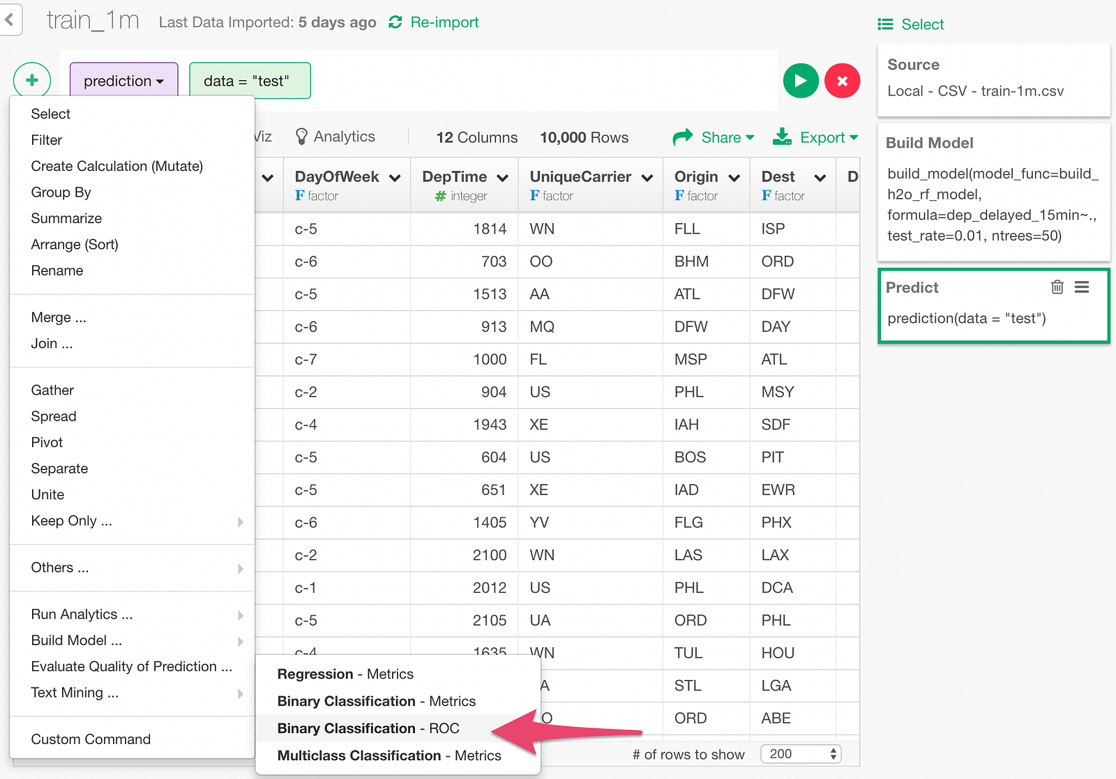
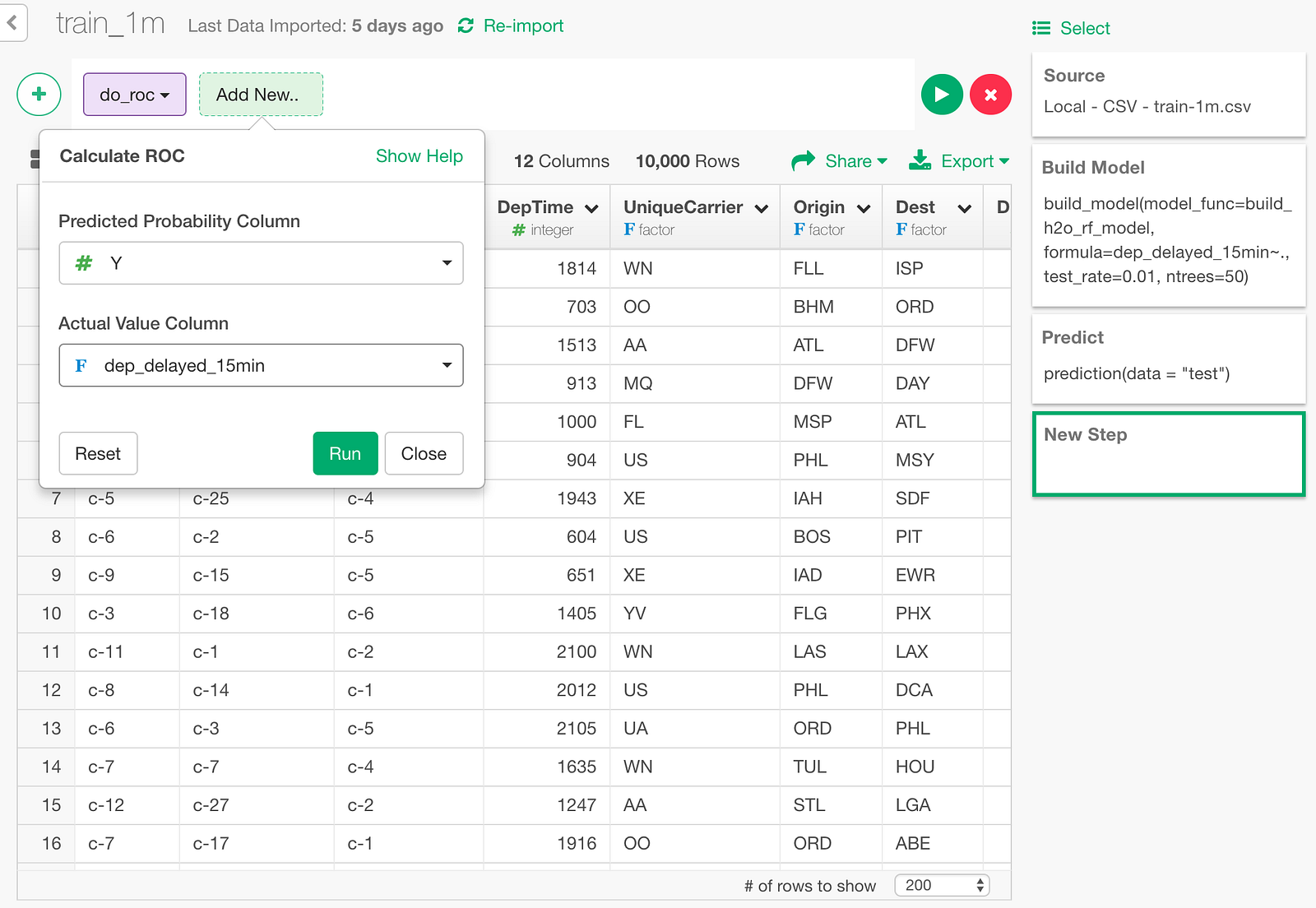
We can also draw ROC curve. Click “Binary Classification — ROC” menu.
In the dialog, specify Y column and dep_delayed_15min column.
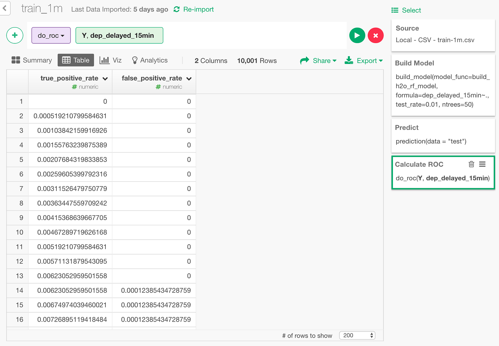
And here is the resulting ROC curve data.
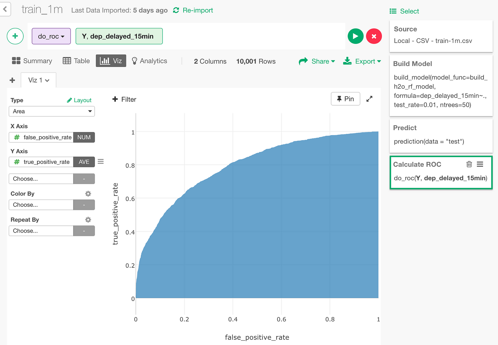
Let’s draw an area chart with this data. The blue area under the ROC curve is the AUC (0.7956) we just looked at.
Summary
As you have seen, we can quickly access the power of H2O by using ‘h2o’ R package and Exploratory’s model extension framework. Thanks to H2O’s multi-process scalable machine learning engine, we can build the predictive models in a much faster speed with bigger data sets.
In the next post, I will compare H2O’s RandomForest against other RandomForest implementation in R such as randomForest and ranger packages, and see how fast H2O really is. Stay tuned!
If you don’t have Exploratory Desktop yet, you can sign up from here for a 30 days free trial. If you are currently a student or teacher, then it’s free!