LightGBM Explained: How It Differs from Random Forest and XGBoost

The evolution of tree-based models - from robustness to optimization to scalability

If you work with tabular data (table data), the kind of structured data found in business analytics, finance, marketing, or operations, you’ve probably encountered three popular machine learning algorithms:

Random Forest
XGBoost
LightGBM

All three rely on decision trees, and they can all produce very strong predictive models. But they were designed with different priorities in mind.

Random Forest emphasizes simplicity and robustness. XGBoost focuses on highly optimized gradient boosting. LightGBM was created to make boosting faster and more scalable.

Understanding why LightGBM was created and how it works makes it much easier to decide whether it’s the right tool for your problem.

The Problem LightGBM Was Designed to Solve

By the mid-2010s, gradient boosting had already proven to be one of the most powerful techniques for predictive modeling on structured data.

In particular, XGBoost had become extremely popular after dominating many machine learning competitions.

However, as datasets continued to grow, practitioners began to encounter new challenges:

datasets with millions of rows
feature sets with thousands of variables
sparse features produced by one-hot encoding
long training times

Gradient boosting was powerful, but it could also be computationally heavy.

Researchers at Microsoft set out to redesign parts of the algorithm so it could handle large datasets more efficiently.

The result was LightGBM, released in 2017.

Why Is It Called “LightGBM”?

LightGBM stands for:

Light Gradient Boosting Machine

The word “Light” does not refer to the speed of light.

Instead, it refers to the algorithm being lightweight in computation and memory usage.

The goal was to create a gradient boosting system that could:

train faster
use less memory
scale to larger datasets

while still maintaining strong predictive performance.

Before diving into LightGBM’s innovations, it helps to understand how the three algorithms differ conceptually.

Random Forest: Many Independent Trees

Random Forest builds many trees independently.

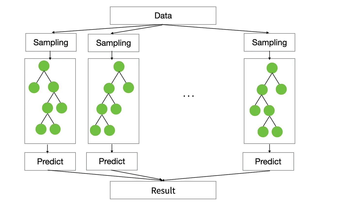
Each tree:

samples the dataset randomly
selects features randomly when splitting
produces its own prediction

The final prediction is simply the average (regression) or majority vote (classification).

Key idea is that many independent trees reduce variance and improve stability compared to a single tree (Decision Tree).

But the trees do not learn from each other.

XGBoost: Trees That Correct Mistakes

XGBoost uses a technique called gradient boosting. Instead of building independent trees, it builds trees sequentially to correct the errors made by the previous trees.

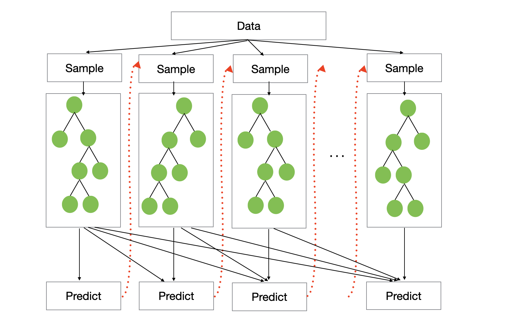
Boosting algorithms are really performing a form of gradient descent in function space.

It builds the first tree and predict and calculate the errors (or loss). If it was a regression problem then the errors can be the residual between the actual and predicted values. And this is called ‘Gradient’.

Row	Actual	Prediction	Gradient (Residual)
1	10	7	3
2	15	14	1
3	8	9	-1

The next tree will be built to predict the gradient values, not the actual values because the gradient tells the model how to move predictions to reduce loss.

And combining the predicted value from the first tree and the predicted values from the second tree will become the new predicted values as a model.

prediction_new = prediction_from_first_tree + learning_rate × prediction_from_second_tree

Conceptually, the model evolves like this:

Tree1 → initial prediction
Tree2 → fix errors from Tree1
Tree3 → fix remaining errors
Tree4 → continue improving

This process usually leads to more accurate models than Random Forest.

However, as datasets grow larger, training boosting models can become computationally expensive.

That is where LightGBM comes in.

LightGBM: Designed to scale

LightGBM does not change the basic idea of gradient boosting.

Instead of optimizing only the boosting algorithm, LightGBM also optimizes:

how trees grow
how rows are sampled
how splits are evaluated
how features are represented

to scale to very large datasets while maintaining strong accuracy.

These improvements come from four key innovations:

Leaf-wise tree growth
Histogram-based splitting
GOSS (Gradient-based One-Side Sampling)
EFB (Exclusive Feature Bundling)

Let’s walk through them one by one.

1. Leaf-Wise Tree Growth

One of the most distinctive features of LightGBM is leaf-wise tree growth.

Traditional tree algorithms such as Random Forest and XGBoost grow trees level-wise.

At each depth of the tree, all nodes are expanded.

Example:

        Root
       /    \
      A      B
     / \    / \
    C   D  E   F

Every level of the tree expands evenly, and it produces balanced trees, which are stable and predictable.

But, they may waste computation expanding branches that do not significantly improve predictions.

LightGBM takes a different approach. Instead of expanding all nodes at the same depth, it expands the leaf that produces the greatest reduction in loss.

Example:

        Root
       /    \
      A      B
     / \
    C   D
   /
  E

The tree grows where the model improves most.

This approach allows LightGBM to reach strong predictive performance with fewer splits.

The trade-off is that trees can become deeper in certain branches, so LightGBM provides parameters such as max_depth and num_leaves to control model complexity.

2. Histogram-Based Splitting

Another important optimization in LightGBM is histogram-based splitting.

Standard tree algorithms may evaluate many possible split thresholds for continuous features.

Example:

Age ≤ 21
Age ≤ 22
Age ≤ 23
Age ≤ 24

LightGBM speeds this up using histogram binning.

Instead of evaluating every unique value, continuous features are grouped into bins.

Example:

Original values:

23, 25, 27, 29, 35

Converted to bins:

20–25
25–30
30–40

Now the algorithm evaluates splits only on bin boundaries.

This dramatically reduces the number of candidate splits and speeds up training.

3. GOSS (Gradient-Based One-Side Sampling)

Training boosting models on large datasets normally requires processing all rows.

LightGBM introduces GOSS (Gradient-based One-Side Sampling) to reduce the number of rows used during training.

The key idea is based on how boosting works.

In boosting algorithms, each data point has a gradient value indicating how much the model needs to adjust its prediction.

Rows with large gradients represent predictions where the model is making large errors.
Rows with small gradients are already well predicted.

While typical boosting algorithms including XGBoost randomly sample the data, LightGBM uses this gradient information to sample the data.

Keeps all rows with large gradients
Keeps only a subset of rows with small gradients

Example:

Dataset: 100,000 rows

Top 20% largest gradients → keep all (20,000 rows)
Remaining 80% → sample 10% (8,000 rows)

This wya, it need to use only 28,000 rows instead of 100,000 rows.

This significantly reduces computation while preserving important learning signals.

4. EFB (Exclusive Feature Bundling)

Many modern datasets contain high-dimensional sparse features, especially when categorical variables are one-hot encoded.

Example:

Row	Red	Blue	Green
1	1	0	0
2	0	1	0
3	0	0	1

These features are mutually exclusive, only one can be active in each row.

Instead of treating them separately, LightGBM bundles them into one feature.

Original:

Row	Red	Blue	Green
1	1	0	0
2	0	1	0
3	0	0	1

Bundled:

Row	ColorBundle
1	1
2	2
3	3

Now the algorithm evaluates splits on one feature instead of three.

This reduces feature dimensionality and speeds up training.

When Should You Use Each Model?

Each algorithm has strengths.

Random Forest

Good when:

you want a simple baseline
datasets are relatively small
minimal tuning is preferred

XGBoost

Good when:

datasets are moderate in size
you want strong predictive performance
stability and extensive tuning options are important

LightGBM

LightGBM works particularly well when:

datasets are large
feature dimension is high
features are sparse
training time matters

Practical Recommendation

A common workflow in machine learning projects is:

Start with Random Forest as a baseline.
Try XGBoost or LightGBM to improve performance.
Prefer LightGBM when datasets become large or training time becomes a bottleneck.

Because of its efficiency and scalability, LightGBM has become a popular choice for many machine learning tasks with tabular data.

Final Thought

Random Forest, XGBoost, and LightGBM all rely on decision trees, but they represent different philosophies:

Random Forest focuses on robust ensembles
XGBoost focuses on optimized gradient boosting
LightGBM focuses on efficient and scalable boosting

Understanding these differences helps you choose the right tool, and explains why LightGBM has become an important algorithm in modern machine learning.

Try LightGBM with Exploratory

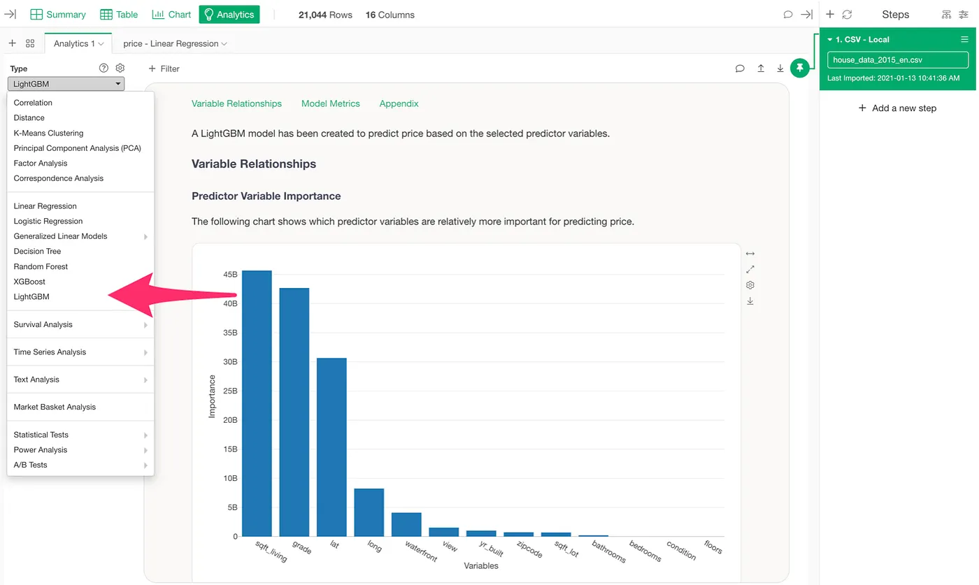
You can try LightGBM with Exploratory v14.5 or later versions.

Go to Analytics view.
Select LightGBM.
Select a Target Variable.
Select Explanatory Variables (Features)
Click Run button.

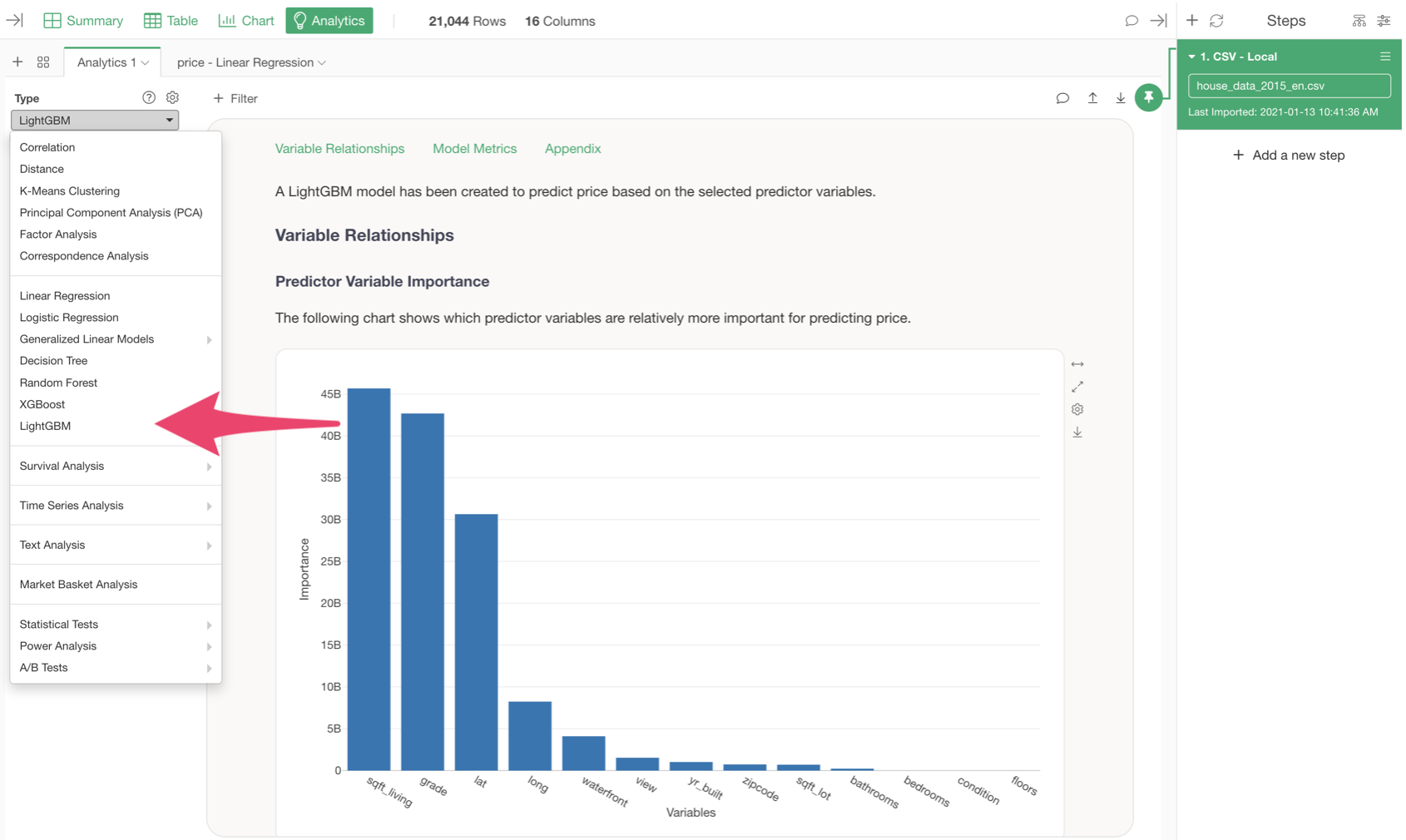
You can take a look at this how-to note for more details on how to use LightGBM.

Download Exploratory

You can start using LightGBM today in the latest version of Exploratory.

👉 Download Exploratory v14

https://exploratory.io/download

If you don’t have an account yet, sign up here to start your 30-day free trial.

https://exploratory.io/

If your trial has expired but you’d like to try the new features, simply launch the latest version and use the Extend Trial option.

If you have questions or feedback, feel free to contact me at kan@exploratory.io .

We’d love to hear how you’re using Exploratory to uncover insights in your data.

Kan Nishida

CEO, Exploratory