Hierarchical Clustering, Explained

Hierarchical clustering puts similar rows into groups and shows all the groups in one tree. Exploratory v16.4 adds it to Analytics. This post explains how the method works, how to read the tree, and how to use it in Exploratory.
Watch the three-minute video first, or read the post. Both explain the same ideas.
Find the groups before you count them
With k-means clustering, you must set the number of clusters before the analysis. Often, you do not know this number yet. You want to see the structure of the data first.
Hierarchical clustering does not need this number. It merges the data points into larger and larger groups, and it records each merge in a tree. You select the number of clusters from the tree after the analysis.
The method is a good fit for small and medium data sets. Examples are 50 stores, 200 products, or 1,000 survey answers.
How the method works
The most common type is agglomerative clustering. It starts with each data point as its own cluster and works from the bottom up. The procedure has six steps:
- Calculate the distance between each pair of data points.
- Put each data point into its own cluster.
- Find the two clusters that have the shortest distance.
- Merge these two clusters into one cluster.
- Calculate the distance from the new cluster to each other cluster.
- Do steps 3 to 5 again until one cluster contains all the data points.
Try it on 14 data points. Click Next step to see each merge. The scatter plot shows the clusters, and the dendrogram on the right records the height of each merge.
Each step merges one pair of clusters. For n data points, the tree has n − 1 merges.
Step 1 needs a distance
Before the first merge, the method must know how far apart two data points are. The most common measure is Euclidean distance. It is the length of a straight line between the two points.
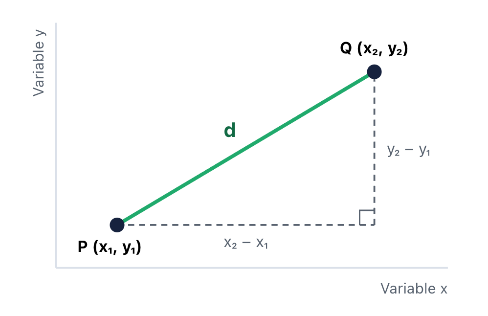
Figure 1. The Euclidean distance d is the length of the straight line from P to Q.
Euclidean distance is the length of a straight line between two data points. For two variables, use this formula:
\[\begin{aligned} d(P, Q) = \sqrt{(x_2 - x_1)^2 + (y_2 - y_1)^2} \end{aligned}\]For more variables, add one squared difference for each variable. Then calculate the square root of the sum.
Other measures are also available. Examples are Manhattan distance and correlation distance.
Standardize your variables first
A variable with large numbers has a large effect on the distance. Look at two customers. They are 30 and 60 years old. Their incomes are $50,000 and $52,000. The age difference is large, and the income difference is small. But with the raw values, income controls the distance.
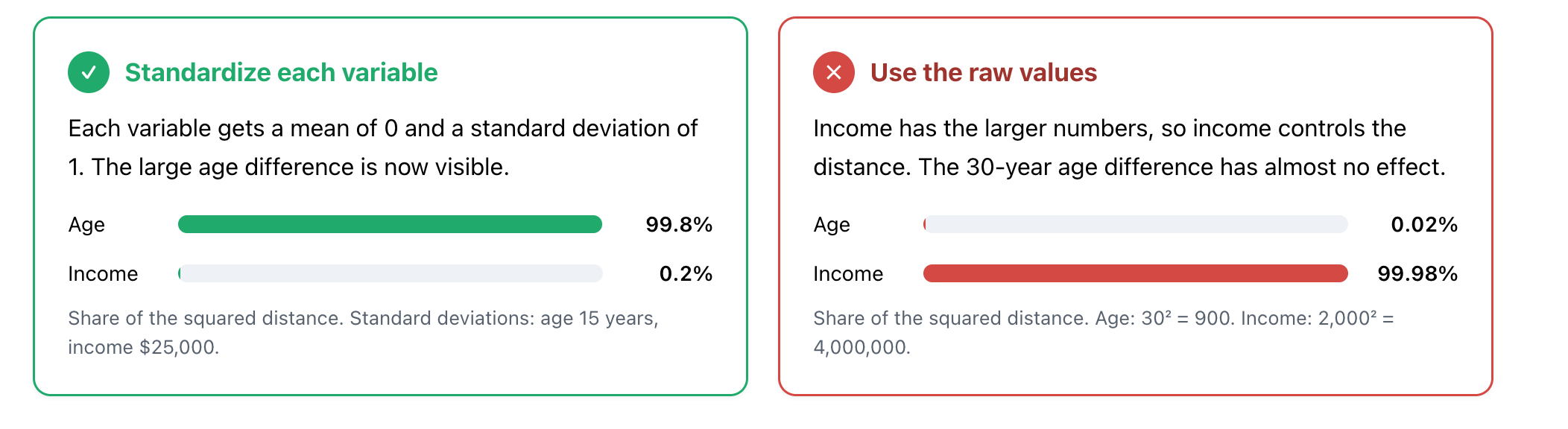
Standardize the variables before you calculate the distances. Exploratory does this by default.
Linkage: the distance between two groups
After the first merge, a cluster can contain many data points. Then the method needs a rule for the distance between two clusters. This rule is the linkage method. There are four common methods.
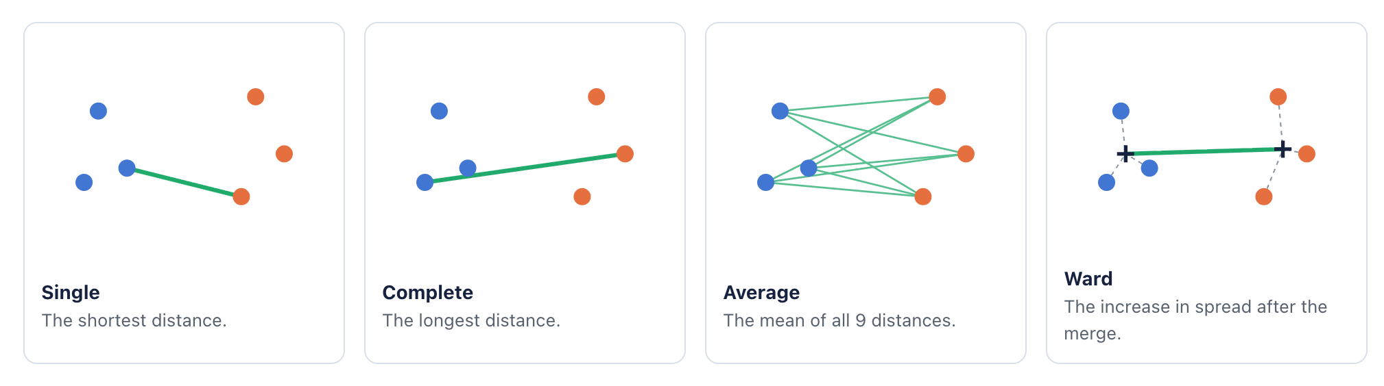
| Method | Distance between cluster 1 and cluster 2 | Typical result |
|---|---|---|
| Single | The shortest distance from a point in cluster 1 to a point in cluster 2. | Long, thin clusters. One noisy point can connect two groups. |
| Complete | The longest distance from a point in cluster 1 to a point in cluster 2. | Compact clusters with similar diameters. |
| Average | The mean of all distances between the points of the two clusters. | A result between single and complete linkage. |
| Ward (Default in Exploratory) | The increase in the within-cluster sum of squares after the merge. | Compact clusters of similar size. |
The choice changes the result. Go back to the explorer, select Single, and click Show all. Point N sits between the lower-left group and the right group. With single linkage, point N acts like a bridge and connects the two groups into one long chain. Ward linkage keeps the three groups separate.
Different linkage methods can give different clusters from the same data. Ward is a good method to start with.
How to read the dendrogram
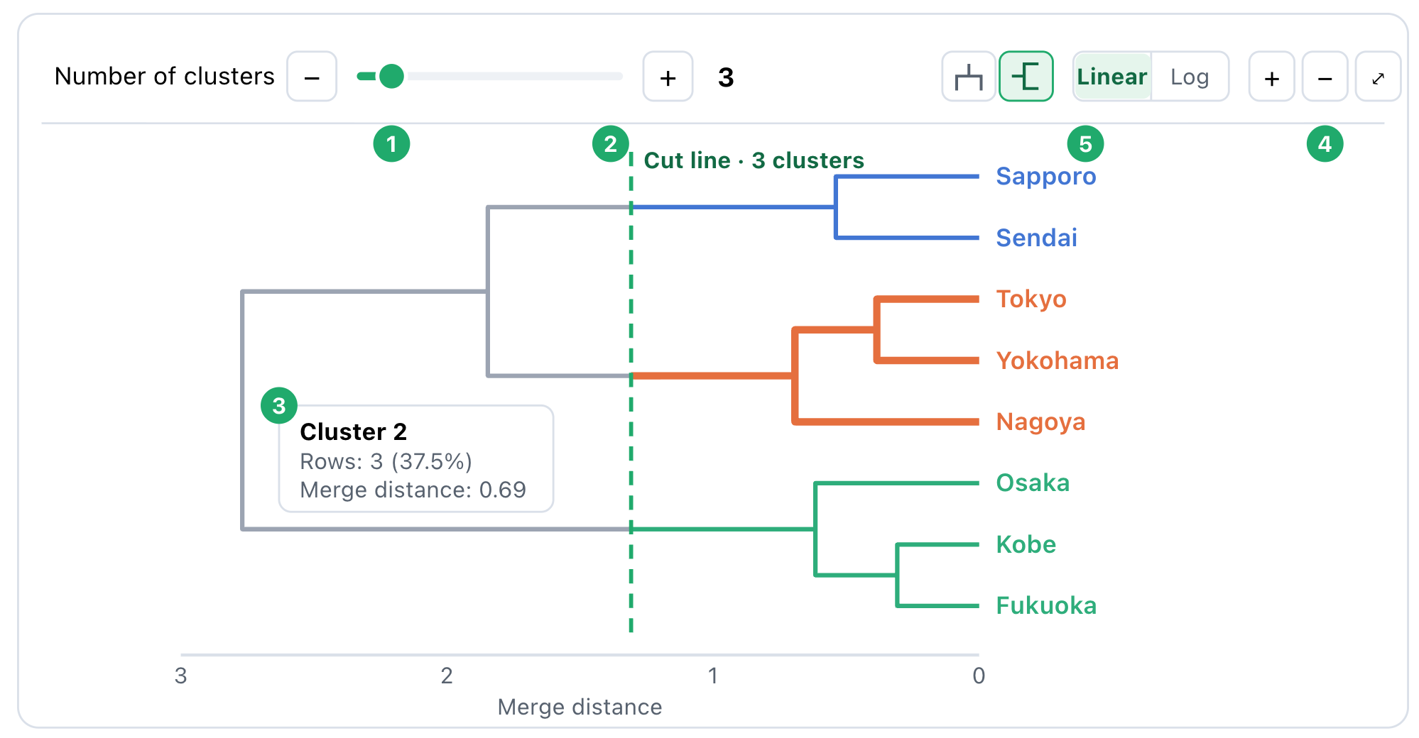
The dendrogram shows all merges in one diagram. The height of each merge is the distance between the two clusters at that merge. To get clusters, you cut the tree with a horizontal line.
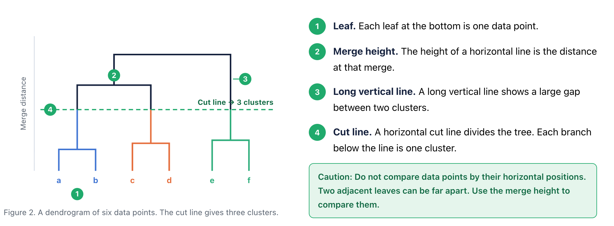
Caution: Do not compare data points by their horizontal positions. Two adjacent leaves can be far apart. Use the merge height to compare them.
Hierarchical clustering or k-means?
Both methods find clusters. They work differently and give different results. Use this table to select a method.
| Item | Hierarchical clustering | K-means clustering |
|---|---|---|
| Number of clusters | Select it after the analysis. | Set it before the analysis. |
| Result | A tree of all merges. | One set of clusters. |
| Same result each time | Yes. | No. The result changes with the random start points. |
| Data size | Small to medium. Memory increases with n². | Large data sets are possible. |
| Cluster shape | Depends on the linkage method. | Round clusters of similar size. |
Try it in Exploratory v16.4
Exploratory v16.4 adds Hierarchical Clustering to Analytics. You do not write code. Exploratory calculates the tree once, and you compare the number of clusters on the dendrogram.
Procedure
- Open the Analytics view of your data frame. Add a new analytics.
- In the type menu, select Clustering Analysis › Hierarchical Clustering.
- For Cluster Target, select Row.
- For Variables, select the numeric columns.
- Optional: For Column for Label, select a column. Its values become the leaf labels.
- Click Run.
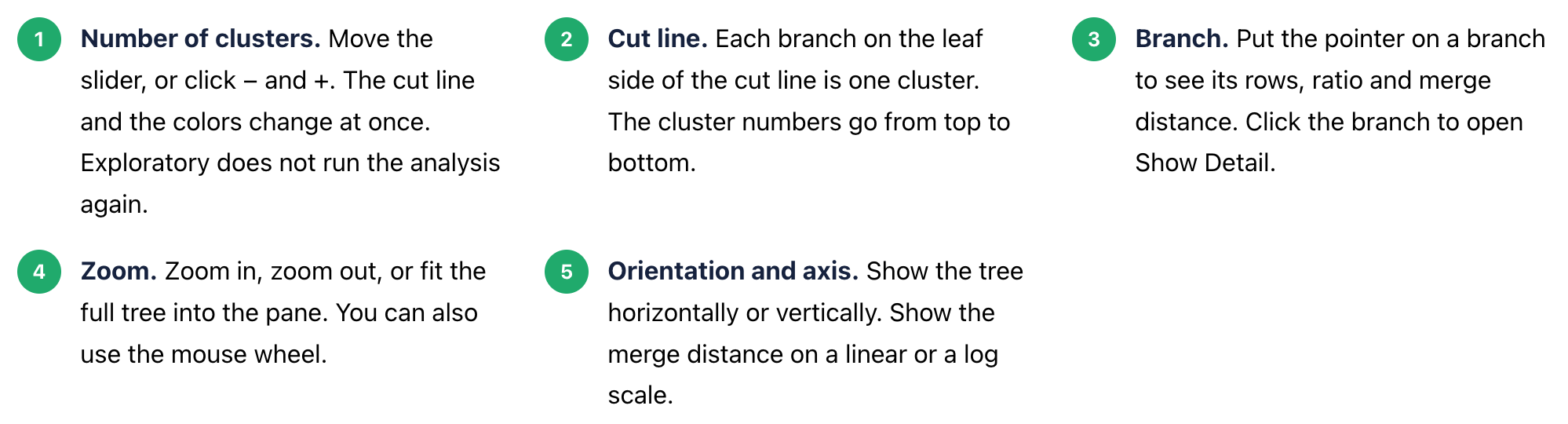
- On the dendrogram, move the Number of clusters slider. Compare the candidates.
- Click a branch. Show Detail opens with the rows of that group.
Cluster Target: Variable puts the variables into clusters, not the rows. The distance is 1 − correlation (Pearson or Spearman). Ward is not available in this mode.
Read the report
After you click Run, Exploratory shows a report with six sections.
| Report section | What it shows |
|---|---|
| Summary | The analysis conditions, and the rows and silhouette scores of each cluster. |
| Cluster Hierarchy | The interactive dendrogram. |
| Choosing Number of Clusters | The Merge Height table. Also the silhouette scores or the elbow curve. |
| Cluster Profile | A radar chart of the cluster means, box plots, and η² for each variable. |
| Cluster Map | The rows in two dimensions, calculated with PCoA from the clustering distances. |
| Output Data | Each row with its cluster. |
Summary
Hierarchical clustering builds one tree that holds every possible grouping.
Standardize the variables before you calculate the distances.
The linkage method changes the shape of the clusters. Ward is a good start.
Cut the tree across long vertical lines.
In Exploratory v16.4, move the slider to compare different numbers of clusters without a new run.
Try Hierarchical Clustering in Exploratory v16.4
Update to Exploratory v16.4. Then open Analytics and select Clustering Analysis › Hierarchical Clustering.