K-Means Clustering, Visually Explained!

K-means clustering puts similar rows of your data into groups. It is fast, and the result is easy to read. This post shows how the method works step by step, when it works well, and how to use it in Exploratory.
Watch the three-minute video first, or read the post. Both explain the same ideas. And, don’t forget to play with the interactive chart below, it shows how K-means create clusters visually!
Find groups in your data
Your data often contains groups of similar rows.
For example, some customers buy often, and other customers buy only with a discount.
In a table with thousands of rows, you cannot see these groups.
K-means clustering finds them for you. You select the number of groups, k. K-means then finds k centers, and puts each row into the group of its nearest center. These groups are clusters.
The center of each cluster is the mean of its rows. This is the reason for the name: k clusters, each with a mean.
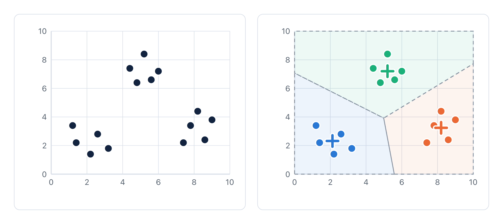
Figure 1. Left: the data before the analysis. Each point is one row with two numeric variables. Right: the result for k = 3. Each center (+) is the mean of its cluster. The dashed lines are the borders between the clusters.
A good result has compact clusters. To measure this, k-means calculates the squared distance from each data point to the center of its cluster. The sum of these values for all clusters is the total within-cluster sum of squares. K-means makes this total as small as possible.
Each cluster has a center, and the center is the mean of its data points. K-means makes the clusters as compact as possible.
How k-means finds the clusters
K-means does not know the clusters at the start. It starts with k centers and improves them step by step. The procedure has only two main steps, and k-means does them again and again.
Select k data points as the start centers.
Put each data point into the cluster of its nearest center.
Move each center to the mean of the data points in its cluster.
Do steps 2 and 3 again. Stop when no data point changes its cluster.
Try it on 15 data points. Click Next step to go through each step. The chart on the right shows the total within-cluster sum of squares after each step. The table under the chart shows the center of each cluster.
With Start 1, two start centers are in the same group. Look at one center as it moves, step by step, to the group that has no center. Select Show the borders to see the area of each center.
Each step decreases the total within-cluster sum of squares, or keeps it the same. K-means stops when no data point changes its cluster.
Why the start centers matter
K-means always stops, but it does not always find the best result. Select Start 2 or Start 3 in the explorer. Each one stops with one group cut in two, and two other groups in one cluster.
At this point, no data point can change its cluster, so k-means cannot correct the result. Compare the final result of each start:
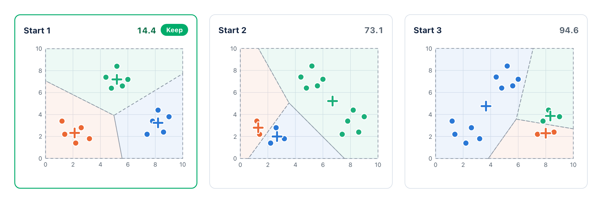
Figure 2. The final result of each start in the explorer, with k = 3. The number is the total within-cluster sum of squares. Smaller is better.
The solution is simple. Run k-means several times from different start centers. Then keep the result with the smallest total within-cluster sum of squares. In the example above, this is the result of Start 1.
In Exploratory, Trial Times sets the number of starts. The default is 1. Exploratory also uses a Random Seed (default 1), so you get the same result each time that you run the analysis.
Tip: Set Trial Times to 10 or more for your final analysis. If the result changes when you change the Random Seed, increase Trial Times.
Use more than one start. Exploratory keeps the start that gives the smallest total within-cluster sum of squares.
Normalize the variables
K-means uses distances, and a distance adds the differences of all variables. If one variable has much larger numbers than the others, that variable controls the result.
Let’s say we have 18 customers with two variables: age in years and
annual income in dollars. There are three groups: young customers, older
customers, and middle-aged customers with a high income.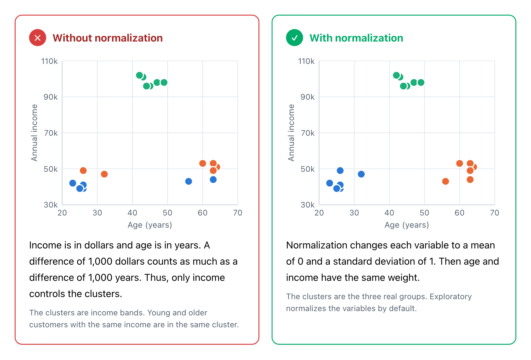
Figure 3. Without normalization, a difference of 1,000 dollars counts as much as a difference of 1,000 years, so only income controls the clusters. Normalization changes each variable to a mean of 0 and a standard deviation of 1.
Normalize the variables when they use different units. In Exploratory, Normalize Variables is TRUE by default.
What k-means cannot find
Each data point goes to its nearest center. Thus, the border between two clusters is always a straight line, halfway between the two centers. This is fast and simple, but it has limits.
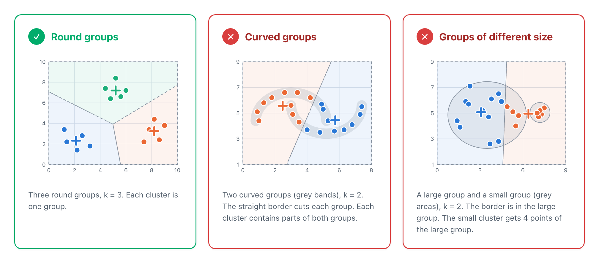
Figure 4. K-means finds round groups of similar size. A straight border cuts curved groups, and moves into a large group next to a small group.
Outliers are also a problem. A data point that is far from all groups pulls the mean of its cluster. For data with outliers, K-Medoids is a better method (see the comparison below).
K-means works best for round groups of similar size. Examine your clusters on a chart. If the groups are curved or of very different sizes, use a different method.
How many clusters?
You set k before the analysis. To select k, run the analysis for a
range of values. Then compare the results with the elbow curve (left
hand side) or with the silhouette score (right hand side). 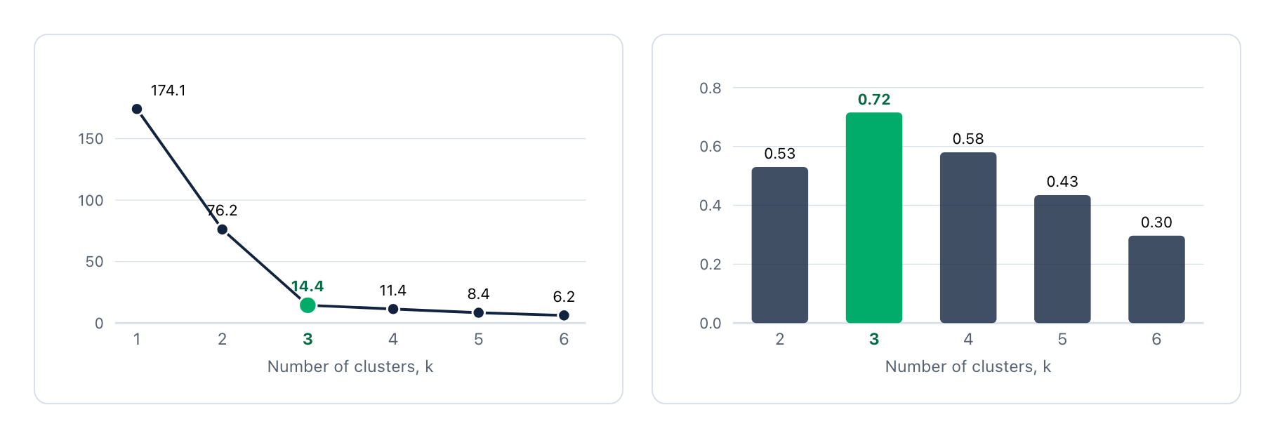
Figure 5. Left: the total decreases quickly to k = 3. After k = 3, the decrease is small. Right: the mean silhouette score is highest at k = 3.
Elbow method. More clusters always give a smaller total within-cluster sum of squares. Thus, do not look for the smallest total. Look for the elbow: the k after which the decrease becomes small.
Silhouette method. For each data point, a is the mean distance to the other points in its cluster. b is the mean distance to the points of the nearest other cluster.
\[\begin{aligned} s(i) = \frac{b - a}{\max(a, b)} \end{aligned}\]A score near 1 shows that the point is in a good cluster. A score less than 0 shows that the point is nearer to another cluster. Select the k with the highest mean score.
Exploratory uses the silhouette method by default. It compares 2 to 10 clusters and shows the scores in the report. You can show the elbow curve by selecting it in the setting.
For the above data, the elbow is at k = 3, and k = 3 also has the highest silhouette score. Also make sure that you can explain the clusters.
K-means, K-medoids or hierarchical clustering?
Exploratory has several clustering methods. Use this table to select a method for your data.
| Item | K-means | K-medoids | Hierarchical clustering |
|---|---|---|---|
| Center of a cluster | The mean. It is usually not a data point. | A medoid. It is a real data point. | No center. The method makes a tree of clusters. |
| Number of clusters | You set k before the analysis. | You set k before the analysis. | You cut the tree after the analysis. |
| Outliers | Large effect on the means. | Small effect on the medoids. | Depends on the linkage method. |
| Values on a scale, for example 1 to 5 | The center can be 3.7, which is not a possible answer. | The center is a possible answer. | No center. |
| Data size | Fast, also for very large data. | Slower. | Slow for large data. It calculates the distance of each pair of rows. |
| Best fit | Large numeric data with round groups. | Survey data and data with outliers. | Small data, when you do not know k. |
Use k-means for large numeric data. Use k-medoids for data with outliers or values on a scale. Use hierarchical clustering to see a tree of all the groups.
Use case: customer segmentation
Customer segmentation is the most common use case for k-means. Each row is one customer. The variables describe the purchases of the customer, for example the number of orders and the order value.
K-means is a good fit for this data. The data is numeric, there are often many rows, and the result is easy to read. Each center is a list of means, one for each variable.
Customer segmentation
Each row is one customer, with four numeric variables about the purchases of the last year. K-means with k = 3 gives three segments.
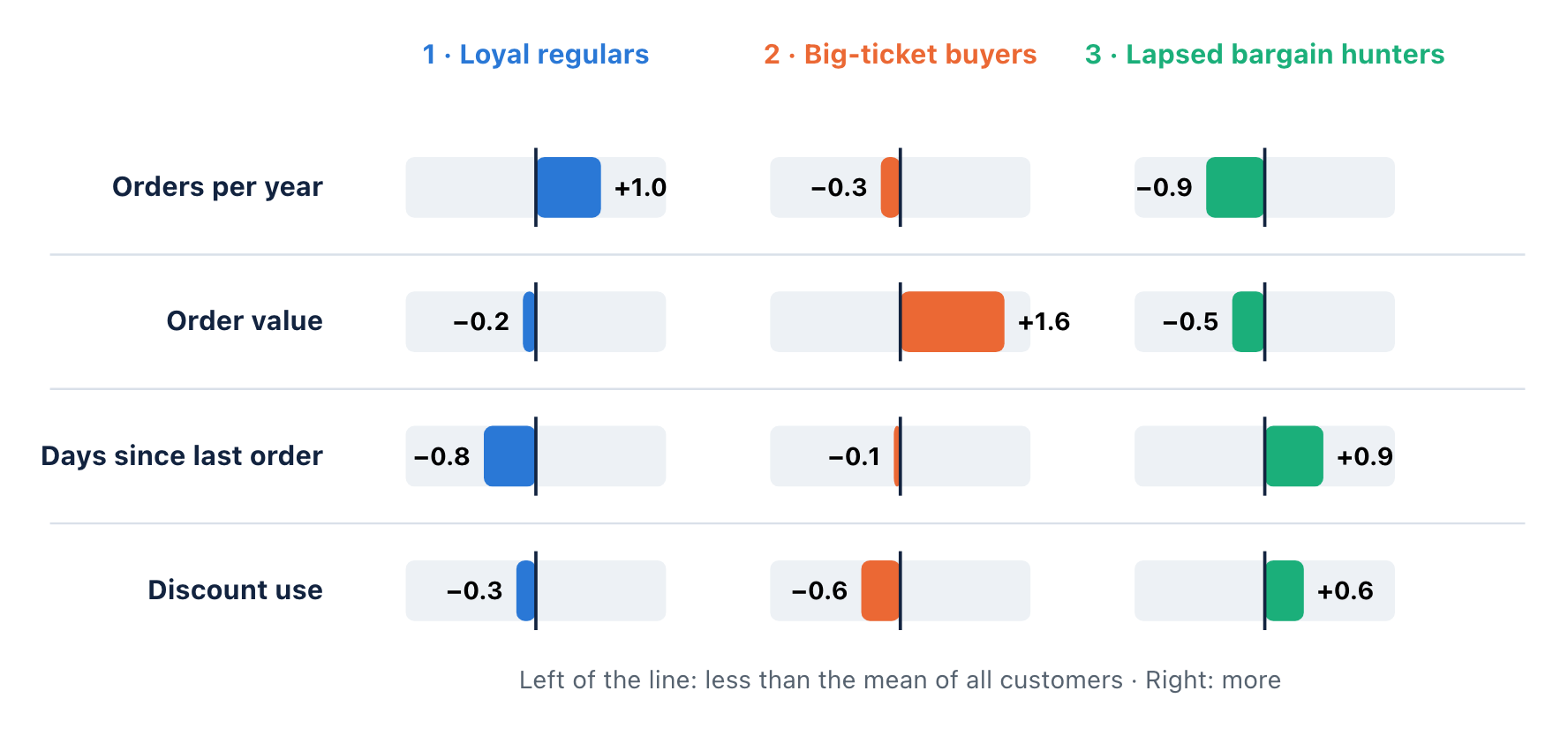
Figure 6. Normalized mean of each variable for each segment. 0 is the mean of all customers. Example data.
| Segment | Customers | Orders per year | Order value | Days since last order | Discount use |
|---|---|---|---|---|---|
| 1 · Loyal regulars | 42% | 10.0 | 74 dollars | 28 | 24% |
| 2 · Big-ticket buyers | 18% | 4.8 | 128 dollars | 56 | 18% |
| 3 · Lapsed bargain hunters | 40% | 2.4 | 65 dollars | 96 | 42% |
| All customers | 100% | 6.0 | 80 dollars | 60 | 30% |
Each segment needs a different action. Thank the loyal regulars. Show new products to the big-ticket buyers. Send an offer to the lapsed bargain hunters before they leave.
Other common use cases
In each case, the data is numeric, and you want a small number of groups with a clear profile.
| Use case | Example data | What k-means gives you |
|---|---|---|
| Customer segmentation (most common) | Orders, order value, days since the last order, discount use. | Segments with a clear profile, for marketing and service. |
| Product or store groups | Sales, margin, size and growth of each product or store. | Groups that need the same plan for price, stock or staff. |
| Usage patterns | Sessions, time of use and features used by each user of an app. | Types of users, for example heavy users and occasional users. |
| Regions and areas | Population, income and age data of each area. | Areas with a similar profile, for a sales plan or a new store. |
| Sensor and machine data | Temperature, pressure and speed of each machine. | Normal operation modes. Points far from all centers can be problems. |
When to use a different method
| Your data or question | Method |
|---|---|
| The values are steps on a scale, for example survey answers from 1 to 5, or the data has outliers. | K-Medoids |
| The values are categories with no order, for example region or yes and no. | K-Modes (Categorical) |
| You do not know the number of clusters, and you want to see a tree of all the groups. | Hierarchical Clustering |
Use k-means to divide many rows of numeric data into a small number of segments. Read the means of each cluster to give each segment a name.
K-Means Clustering in Exploratory
Exploratory has K-Means Clustering in Analytics. You can use its UI to generate a report to show the result. Exploratory internally uses the kmeans function of R.
Procedure
Open the Analytics view of your data frame. Add a new analytics.
In the type menu, select Clustering Analysis › K-Means (Numerical).
For Variables, select the numeric columns.
(Optional) Open the settings. Set the Number of Clusters and the Trial Times.
Click Run.
Default Settings: 3 clusters, the Hartigan-Wong algorithm, 1 trial, Random Seed 1 and normalized variables. The silhouette method compares 2 to 10 clusters.
Hartigan-Wong is a refined version of the procedure above. It moves one data point at a time to another cluster when this move decreases the total within-cluster sum of squares. It usually finds a result that is as good as, or better than, the result of the basic procedure.
What the results look like
The example uses an employee survey with seven questions about work. The analysis uses the default of 3 clusters.
In Choosing Number of Clusters, compare the
silhouette scores. If necessary, change the Number of Clusters and run
again.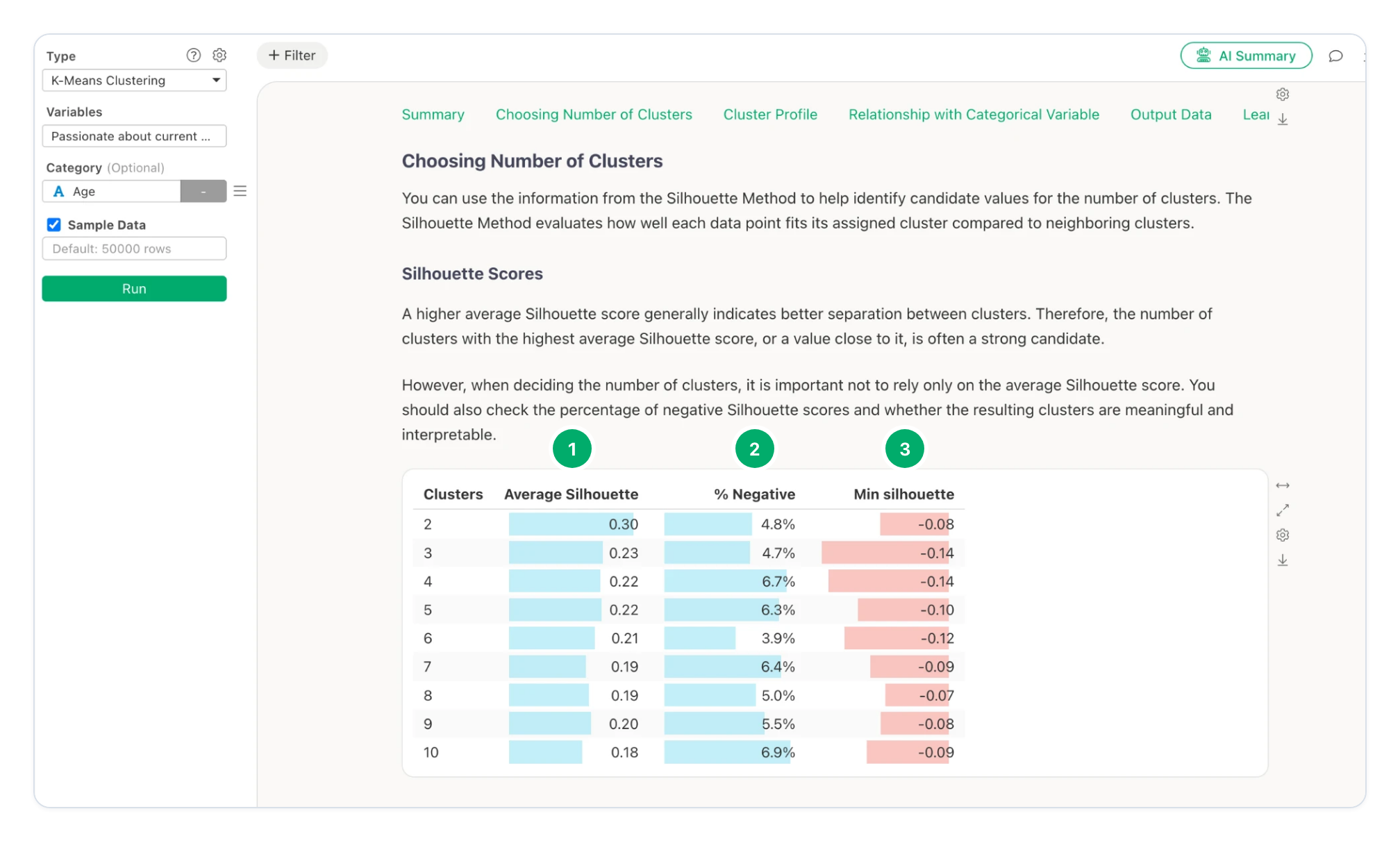
Figure 7. Choosing Number of Clusters › Silhouette Scores for 2 to 10 clusters. Screenshot from Exploratory.
Average Silhouette. The mean silhouette score for each number of clusters. Here, 2 clusters have the highest score, 0.30. 3 clusters have 0.23.
% Negative. The percentage of rows that are nearer to another cluster. It stays low, from 3.9% to 6.9%.
Min silhouette. The lowest silhouette score of one row for each number of clusters.
Note: Survey data often gives low silhouette scores, because the answers of different people overlap. Do not select the number of clusters from the score only. Here, 3 clusters have a lower score than 2 clusters (0.23 and 0.30), but the three clusters are easy to explain, as the next charts show.
In Cluster Profile, examine how the clusters are
different.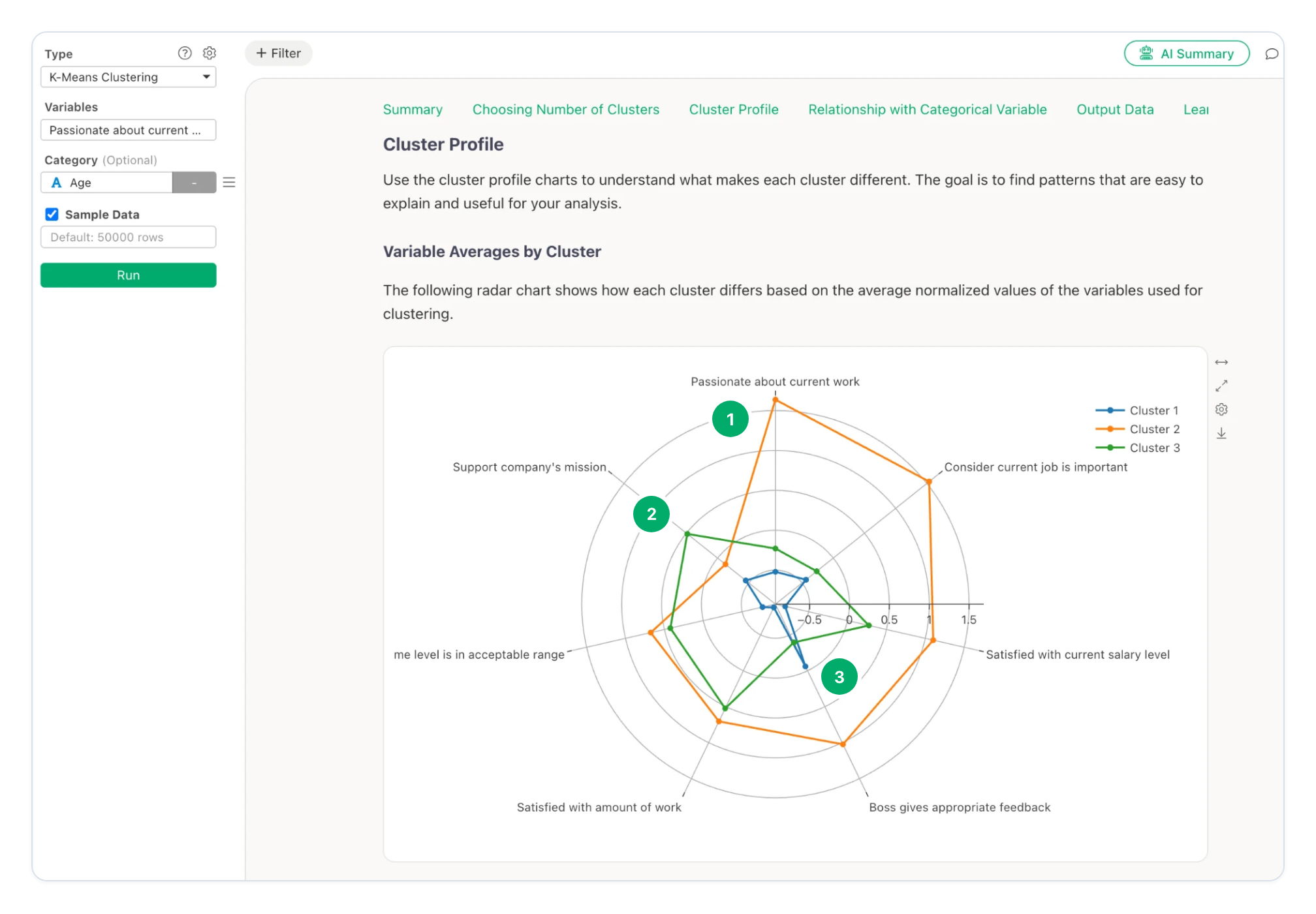
Figure 8. Cluster Profile › Variable Averages by Cluster. The values are normalized: 0 is the mean of all rows. Screenshot from Exploratory.
Cluster 2. Much higher than the mean for “Passionate about current work” and “Consider current job is important”. Also high for salary and feedback from the boss.
Cluster 3. Higher than the mean for “Support company’s mission”, the amount of work and the overtime level. Lower than the mean for passion.
Cluster 1. Lower than the mean for almost all questions. Only “Boss gives appropriate feedback” is near the mean.
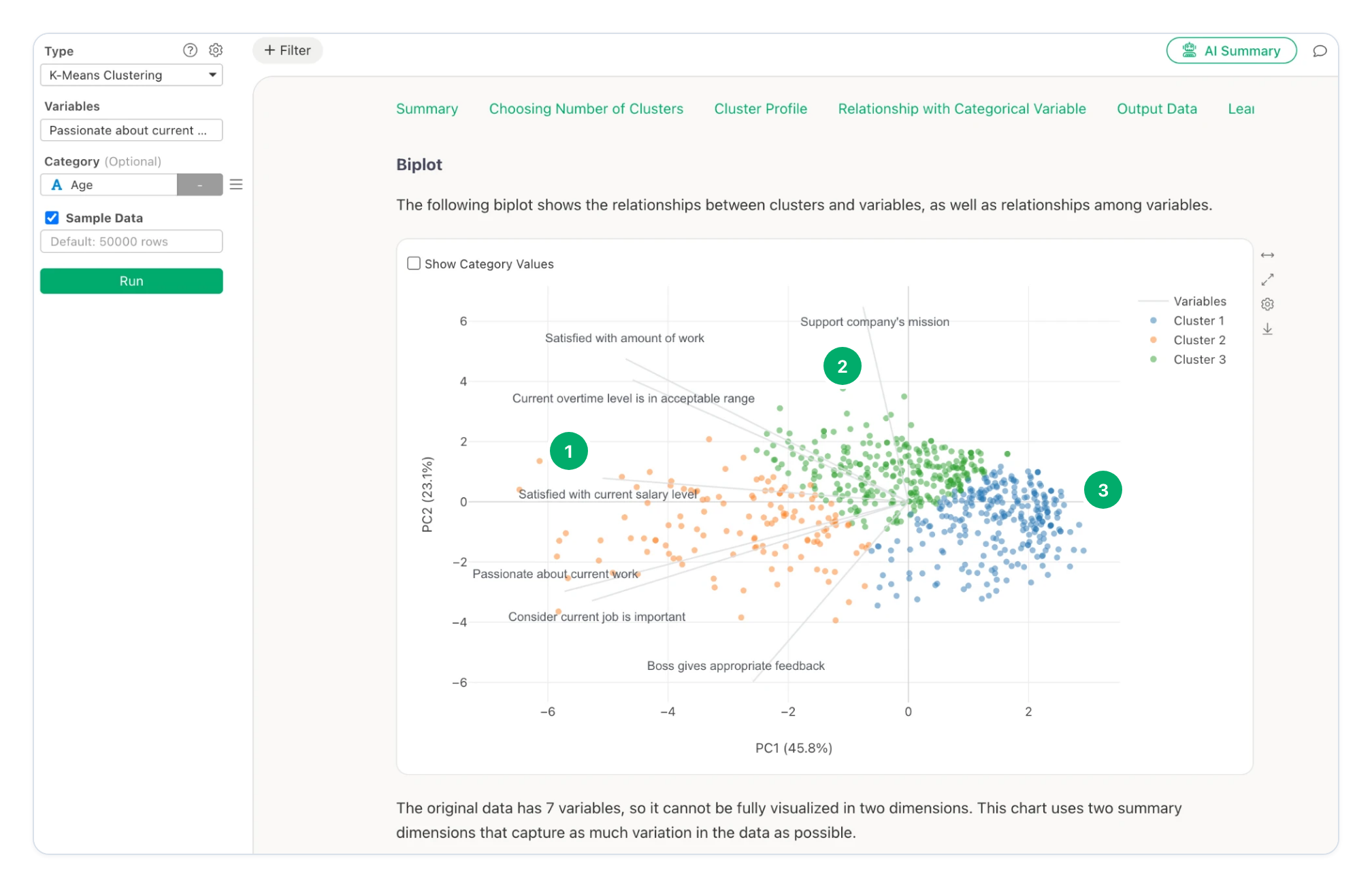
Figure 9. Cluster Profile › Biplot. Each point is one row. Each grey line is one question. Screenshot from Exploratory.
Cluster 2 is on the left, in the direction of the lines for passion, job importance and salary.
Cluster 3 is at the top, in the direction of the lines for the company’s mission, the amount of work and overtime.
Cluster 1 is on the right, opposite to all lines. These rows have low values for most questions.
In this example, cluster 2 is the engaged employees. Cluster 3 is satisfied with the work conditions, but is not passionate about the work. Cluster 1 is not satisfied with most items. Each cluster needs a different action from the company.
Read the report
After you click Run, Exploratory shows a report with these sections.
| Report section | What it shows |
|---|---|
| Summary | The analysis conditions. For each cluster: rows, ratio, sum of squares and silhouette scores. Also the average values by cluster and the rows that the analysis excluded. |
| Choosing Number of Clusters | The silhouette scores, or the elbow curve and the reduction in variation. |
| Cluster Profile | A radar chart of the averages, the variation in each cluster, the variables that characterize the clusters (eta-squared) and a biplot. |
| Relationship with Categorical Variable | How the values of a category column are distributed across the clusters. Only when you select a category column. |
| Output Data | Each row of the data with its cluster. |
Summary
K-means puts each data point into the cluster of its nearest center. Each center is the mean of its cluster.
The procedure puts the points into clusters, then moves the centers. It does these two steps again until no point changes its cluster.
A poor start can give a poor result. Increase Trial Times to try more starts.
Normalize the variables when they use different units. K-means works best for round groups of similar size.
Compare the silhouette scores, but select a number of clusters that you can explain.
Try It with Exploratory
Try K-Means Clustering with your own data in Exploratory.
👉 Download the latest version of Exploratory
https://exploratory.io/download
If you do not have an Exploratory account, sign up and start a 30-day free trial here:
If your trial has expired, launch the latest version and click Extend Trial to try it again.