K-Medoids Clustering, Visually Explained

K-medoids clustering puts similar rows into groups. The center of each group is a real row of your data. This post explains how the method works, why it is a good fit for survey data, and how to use it in Exploratory.

Watch the three-minute video first, or read the post. Both explain the same ideas.

https://www.youtube.com/watch?v=bUxDL_PiVYc

A cluster center that you can read

K-means clustering is the most common clustering method. It gives each cluster a center, and this center is the mean of the cluster. The mean is a calculated position. Usually, no row of your data is at this position.

This is a problem when you want to describe a cluster. Example: a survey asks questions on a scale of 1 to 5. The mean of a cluster can be 3.7, but no respondent can give the answer 3.7.

K-medoids clustering solves this problem. It uses one of the rows as the center of each cluster. This row is the medoid. It is the row with the smallest total distance to the other rows of its cluster.

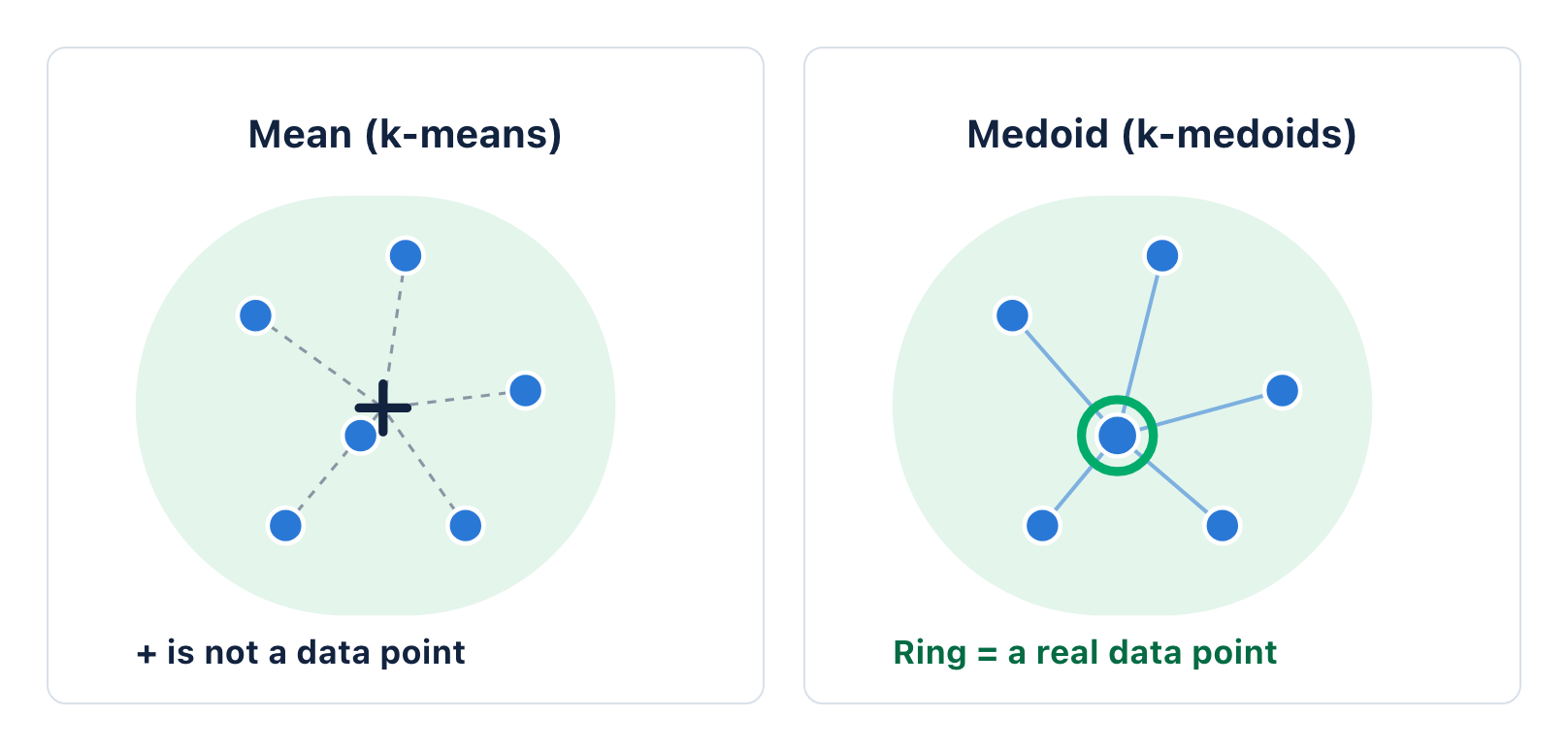
Left: six data points with their mean, a cross that is not on a data point. Right: the same points, where one data point, the medoid, has a green ring.

Figure 1. Left: the mean (+) is a calculated position. Right: the medoid (ring) is the data point with the smallest total distance to the other points in its cluster.

Each cluster has a medoid. A medoid is a real row of your data, so you can read it as a typical example of the cluster.

How PAM finds the medoids

The most common algorithm for k-medoids is PAM (Partitioning Around Medoids). It makes the total distance from each row to its medoid as small as possible. PAM has two phases. The BUILD phase selects a good set of start medoids. The SWAP phase then replaces medoids while the total distance decreases.

Build phase

Calculate the distance between each pair of data points.
Select the data point with the smallest total distance to all other points. This point is the first medoid.
Add the data point that decreases the total distance most. Do this step again until there are k medoids.

Swap phase

Put each data point into the cluster of its nearest medoid.
For each medoid and each other data point, calculate the total distance after you swap them.
If the best swap decreases the total distance, make that swap. Then do steps 4 to 6 again.
Stop when no swap decreases the total distance.

Try it on 14 data points. Click Next step to go through each step. The label above the charts shows the phase and the step of the procedure. In each SWAP round, the explorer first shows all the swaps that PAM tries. Then it makes the best swap and puts each point into a cluster again.

With the BUILD start, the medoids are almost correct before the SWAP phase starts. Select Poor start to see a longer SWAP phase. All three start medoids are then in the same group, and SWAP needs three rounds to correct them.

Each swap decreases the total distance. PAM stops when no swap can decrease it. From the poor start, SWAP finds the same medoids as from the BUILD start.

Why a real center matters

A mean moves toward extreme values. A medoid does not, because it must be one of the rows. In the example below, customer G spends 1,000 each month. The other six customers spend between 120 and 175. The mean moves to 269, which is higher than the spend of 6 of the 7 customers. The medoid stays at 150, with customer D.

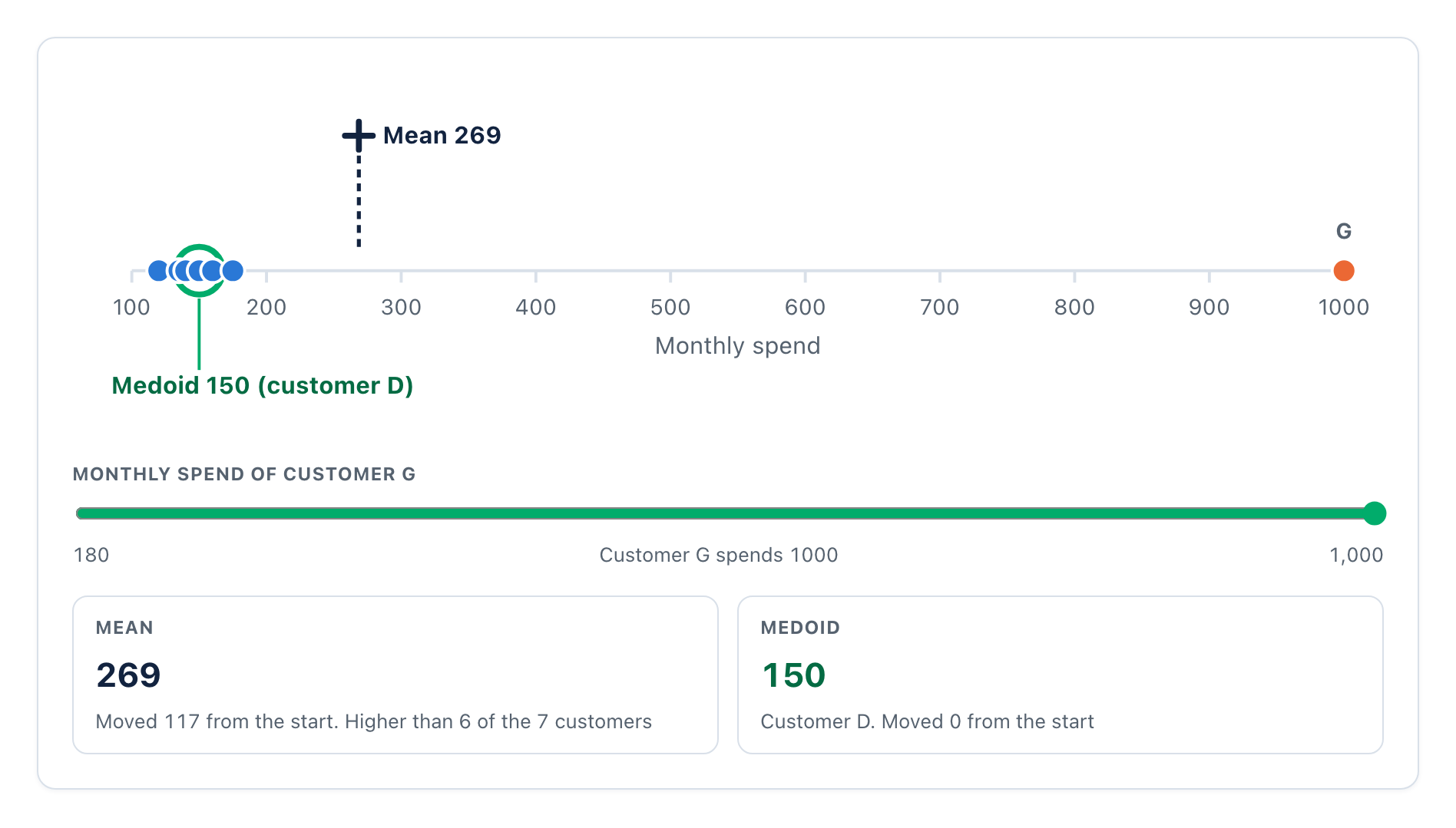
Number line of the monthly spend of seven customers. Customer G spends 1,000. The mean is 269. The medoid is customer D at 150.

Figure 2. When customer G spends 1,000, the mean moves from 151 to 269. The medoid stays at 150.

Read the center of a cluster

The same difference is important when the values are steps on a scale. Look at the center of one cluster of survey respondents. Each respondent answered three questions on a scale of 1 to 5.

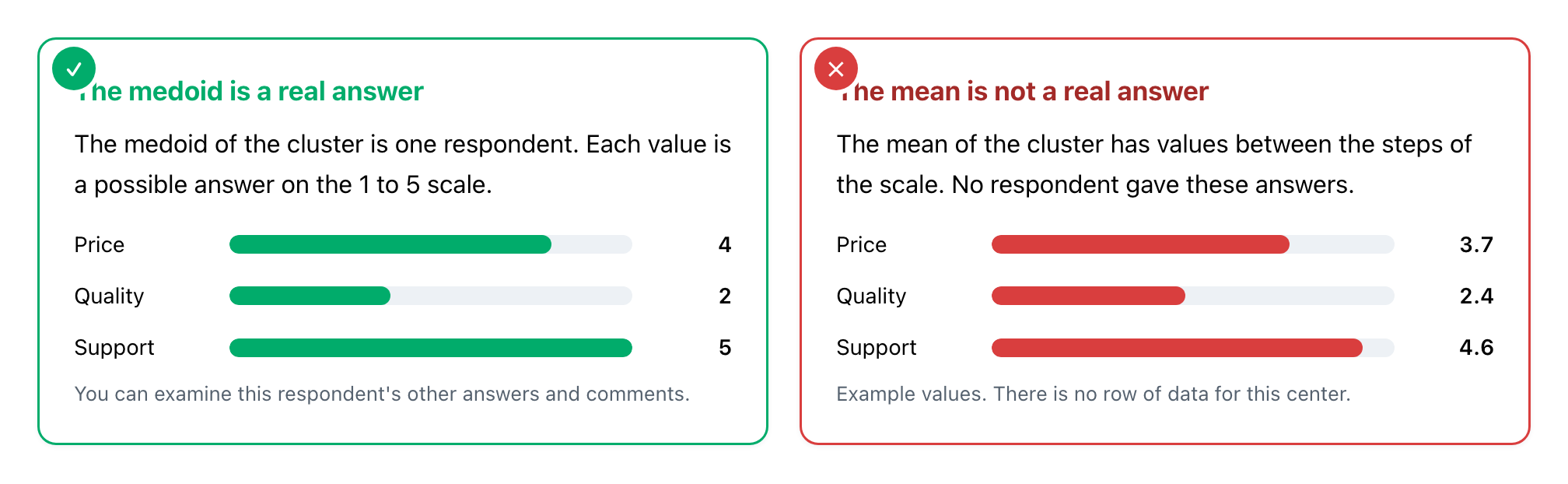
Good: the medoid is a real answer, 4, 2 and 5. Bad: the mean is not a real answer, 3.7, 2.4 and 4.6.

Figure 3. The medoid of the cluster is one respondent with possible answers. The mean has values between the steps of the scale. Example values.

Use k-medoids when your data has outliers, or when the values are steps on a scale. The center of each cluster stays a real, possible row.

Manhattan or Euclidean distance

K-medoids uses only the distances between rows. It never calculates a mean. Thus, it can use many distance measures. The two most common measures are Manhattan distance and Euclidean distance.

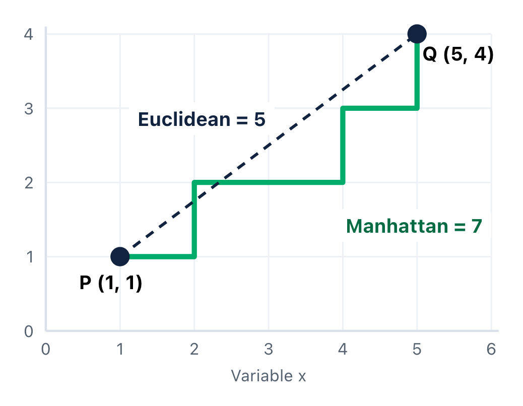
Grid with points P (1, 1) and Q (5, 4). A green staircase path shows the Manhattan distance 7. A dashed straight line shows the Euclidean distance 5.

Figure 4. From P to Q, the Manhattan distance is 4 + 3 = 7. The Euclidean distance is 5.

Manhattan distance is the sum of the absolute differences of each variable. The path follows the grid, like the streets of a city.

\[\begin{aligned} d(P, Q) = |x_2 - x_1| + |y_2 - y_1| \end{aligned}\]

Euclidean distance is the length of a straight line between two data points.

\[\begin{aligned} d(P, Q) = \sqrt{(x_2 - x_1)^2 + (y_2 - y_1)^2} \end{aligned}\]

Euclidean distance squares each difference. Thus, one large difference has a large effect. Manhattan distance does not square the differences, so outliers have less effect.

Note: Standardize the variables before you calculate the distances. Then a variable with large numbers does not control the result.

Use Manhattan distance when your data has outliers or values on a scale. Exploratory uses Manhattan distance by default.

How many clusters?

You set the number of clusters, k, before the analysis. To select k, run the analysis for a range of values. Then compare the results with the silhouette score or with the elbow curve.

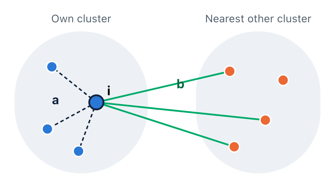
Point i in the blue cluster. Distance a goes to the other blue points. Distance b goes to the points of the nearest other cluster.

Figure 5. a is the mean distance from point i to the other points in its cluster. b is the mean distance to the points of the nearest other cluster.

The silhouette score of one data point is:

\[\begin{aligned} s(i) = \frac{b - a}{\max(a, b)} \end{aligned}\]

Near 1. The point is near its own cluster and far from the other clusters.
Near 0. The point is on the border between two clusters.
Less than 0. The point is nearer to another cluster. It is possibly in the wrong cluster.

Calculate the mean silhouette score of all points for each k. Select the k with the highest mean score, or a k with a score near to it that gives clusters you can explain.

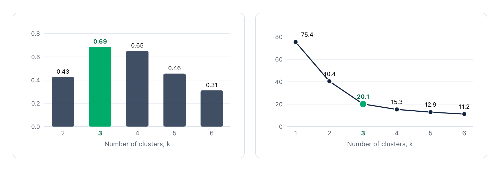
Left: mean silhouette score for k from 2 to 6, highest at k = 3 with 0.69. Right: total distance to the medoids for k from 1 to 6, with a bend at k = 3.

Figure 6. Left: mean silhouette score of the 14 explorer points. Right: total distance to the medoids. Both use Manhattan distance.

For the 14 points of the explorer, k = 3 has the highest silhouette score. The elbow curve also bends at k = 3.

Large data: PAM and CLARA

PAM is exact, but it is slow for large data. In each SWAP round, it examines k × (n − k) swaps, and each swap needs the distances of all n rows. CLARA (Clustering LARge Applications) is a faster method. It runs PAM on small samples of the rows. Then it keeps the medoids that give the smallest total distance on all rows.

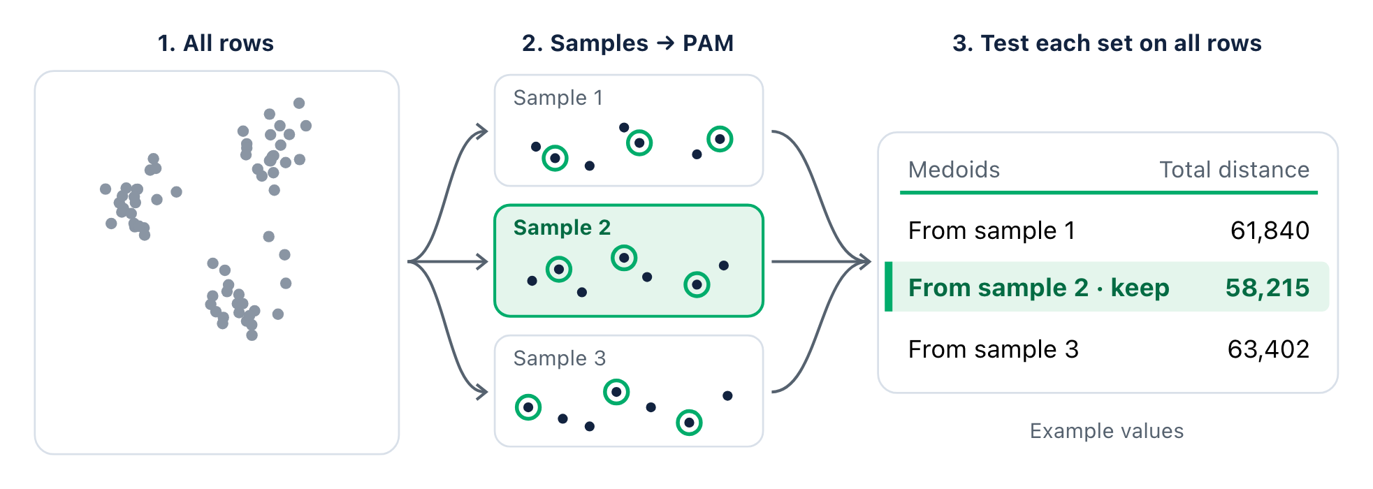
CLARA: draw samples from all rows, run PAM on each sample, test each set of medoids on all rows, and keep the best set.

Figure 7. CLARA runs PAM on small samples. It keeps the medoids that give the smallest total distance on all rows. The total distances are example values.

Item	PAM	CLARA
Data used for the search	All rows.	Several random samples of the rows.
Result	The best medoids that the swap search finds.	An approximate result. More samples give a more stable result.
Time	Increases quickly with the number of rows.	Increases slowly with the number of rows.
In Exploratory (Auto, the default)	Used for 5,000 valid rows or fewer.	Used for more than 5,000 valid rows.

Use PAM for small and medium data. Use CLARA for large data. In Exploratory, the Auto setting selects the algorithm for you.

K-medoids or k-means?

Both methods divide the data into k clusters. The difference is the center of each cluster. Use this table to select a method.

Item	K-medoids clustering	K-means clustering
Center of a cluster	A medoid. It is a real data point.	A mean. It is usually not a data point.
Distance	Many measures. Exploratory has Manhattan and Euclidean.	Squared Euclidean distance.
Outliers	Small effect on the medoids.	Large effect on the means.
Values on a scale	The center is a possible answer, for example 4 on a 1 to 5 scale.	The center can be 3.7, which no respondent gave.
Same result each time	Yes, with the BUILD start of PAM.	No. The result changes with the random start points.
Data size	Small to medium with PAM. Large with CLARA.	Large data sets are possible.

Use case: survey data

Survey data is the most common use case for k-medoids. Many surveys ask people to agree or disagree on a scale of 1 to 5. This is a Likert scale. The answers are ordered categories, not exact quantities.

The table below shows nine respondents in three clusters. The first row of each cluster is its medoid. Under each cluster, the cluster mean has values such as 4.3 and 1.7. No respondent can give these answers.

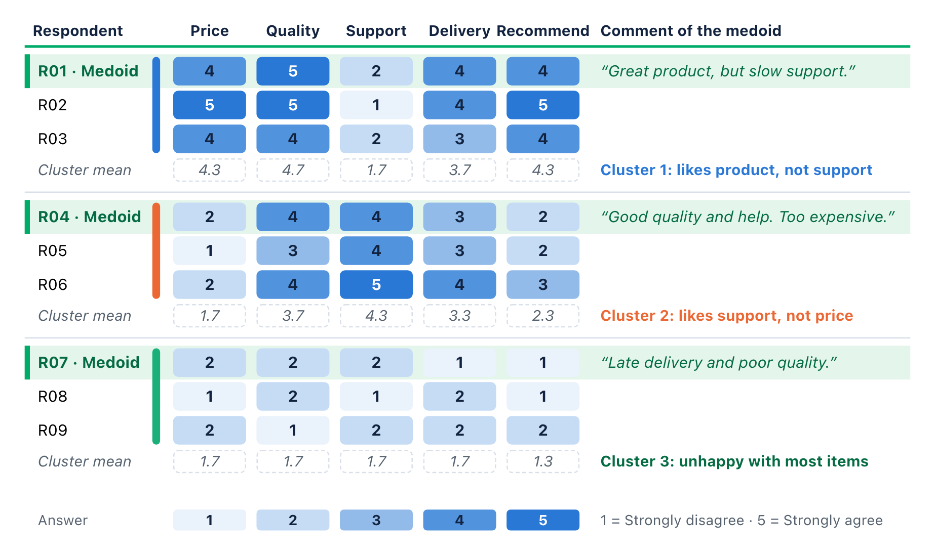
Nine survey respondents and five questions on a 1 to 5 scale, in three clusters. The first row of each cluster is the medoid, with a comment. Under each cluster, the cluster mean has values such as 4.3 and 1.7.

Figure 8. Nine respondents in three clusters, with Manhattan distance. The medoid of each cluster is one real respondent. The cluster means have values that no respondent can give. Example data.

Why k-medoids fits survey data

A real answer pattern. Each value of a medoid is a step on the scale. You can report the medoid as it is.
Steps, not squares. Manhattan distance adds the number of steps between two answers. A difference of 2 steps counts as 2, not 4.
Extreme respondents. Some respondents select only 1 or only 5. They have a small effect on the medoids.
A real person. The medoid is one respondent. Read the comments and the profile of this respondent to describe the cluster.

Prepare survey data

Give each answer a number, from 1 = Strongly disagree to 5 = Strongly agree.
Make sure that each question column is numeric. K-Medoids in Exploratory accepts only numeric variables.
Make sure that all questions have the same direction. For a negative question, calculate 6 − answer.
If all questions use the same scale, you can set Standardize Variables to FALSE. Then the distance counts the steps on the scale.

Other common use cases

K-medoids is also useful in other areas. The two reasons are the same in each case: a real row as the center, and a small effect from outliers.

Use case	Example data	What k-medoids gives you
Survey and feedback analysis (most common)	Customer satisfaction, employee engagement and product feedback on a 1 to 5 scale.	Centers that are possible answers. One real respondent for each cluster.
Customer segmentation with outliers	Spend, number of orders and days since the last order. A few customers spend very much.	Centers that the large customers do not pull. One real customer to examine for each segment.
Representative stores or sites	Stores or warehouses with their sales, size and location.	One real store for each cluster. Use it as a test store, or as a model for the other stores.
Typical cases for review	Products, patient records or support tickets with numeric attributes.	k real cases to read, one for each cluster, not k averages.
Data with measurement errors	Sensor values with sudden spikes.	Medoids that the spikes do not move.

When to use a different method

Your data or question	Method
The answers are categories with no order, for example region or yes and no.	K-Modes (Categorical)
Many rows of numeric data with no outliers, and you do not need a real row as the center.	K-Means
You do not know the number of clusters, and you want to see a tree of all the groups.	Hierarchical Clustering

Use k-medoids for survey data on a Likert scale. Each cluster then has a real respondent as its typical example.

Try it in Exploratory

Exploratory has K-Medoids Clustering in Analytics. You do not write code. Exploratory uses the PAM and CLARA algorithms of the R package cluster.

Procedure

Open the Analytics view of your data frame. Add a new analytics.
In the type menu, select Clustering Analysis › K-Medoids (Ordinal / Numerical).
For Variables, select the numeric columns.
Open the settings. Set the Number of Clusters.
Click Run.
In Choosing Number of Clusters, compare the silhouette scores. If necessary, change the Number of Clusters and run again.
In Medoid Details, examine the medoid row of each cluster.

What the results look like

The example uses a survey about coffee products. It has 16 questions on a scale of 1 to 5. The analysis uses the default of 3 clusters.

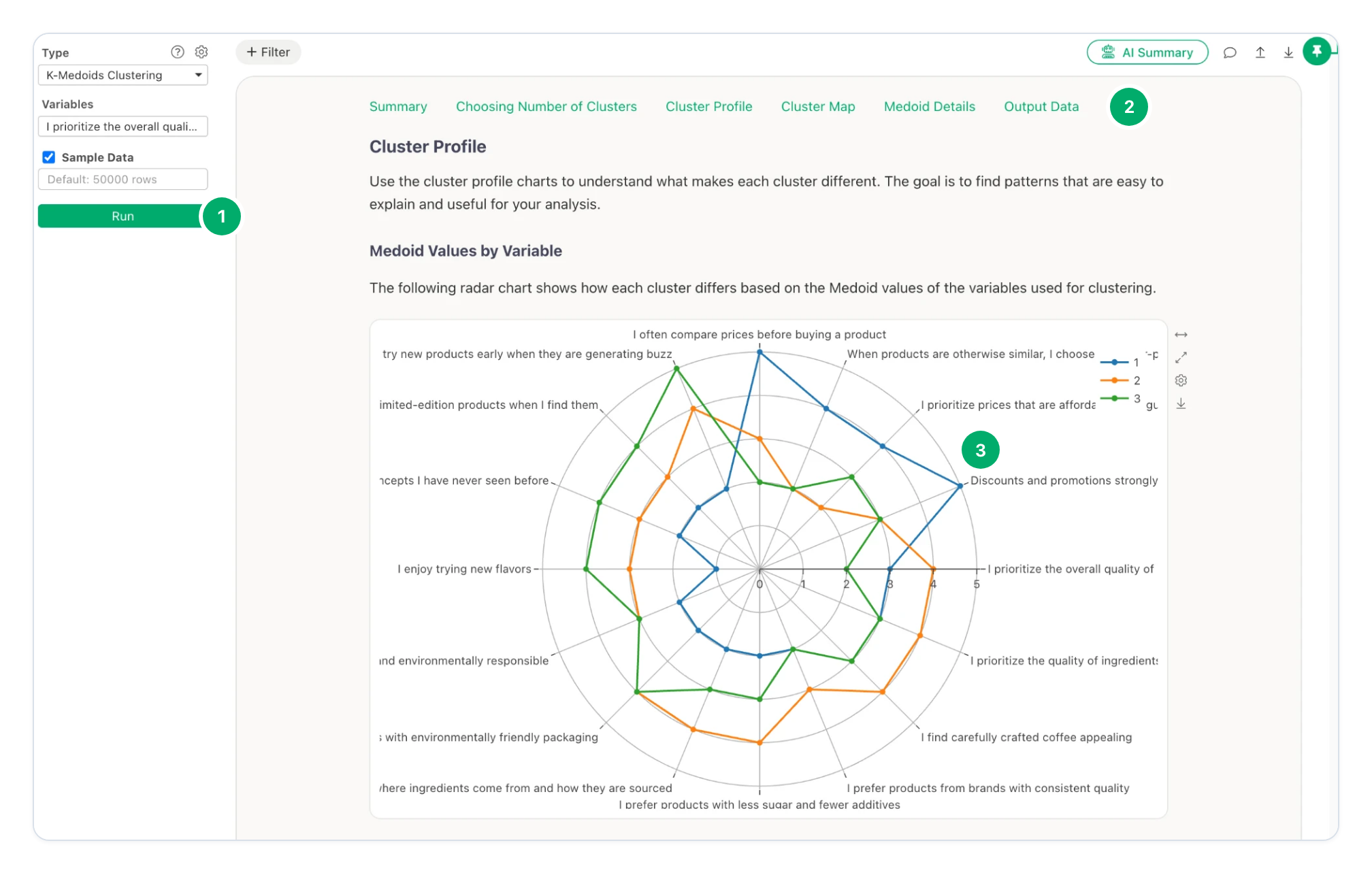
Exploratory with K-Medoids Clustering selected as the Type. The Cluster Profile section shows a radar chart of the medoid values of three clusters for 16 survey questions.

Figure 9. Cluster Profile › Medoid Values by Variable. Each line is the medoid of one cluster, which is one real respondent. Screenshot from Exploratory.

Settings. For Type, select K-Medoids Clustering. For Variables, select the question columns. Then click Run.
Report sections. The report has six sections. The table below shows what each section contains.
Medoid line. The medoid of cluster 1 gives 5 to “Discounts and promotions” and to “I often compare prices”. Each point is a real answer.

In this example, cluster 1 gives high answers to the price questions. Cluster 2 gives high answers to the quality questions, for example ingredients and less sugar. Cluster 3 gives high answers to the questions about new products, new flavors and limited editions.

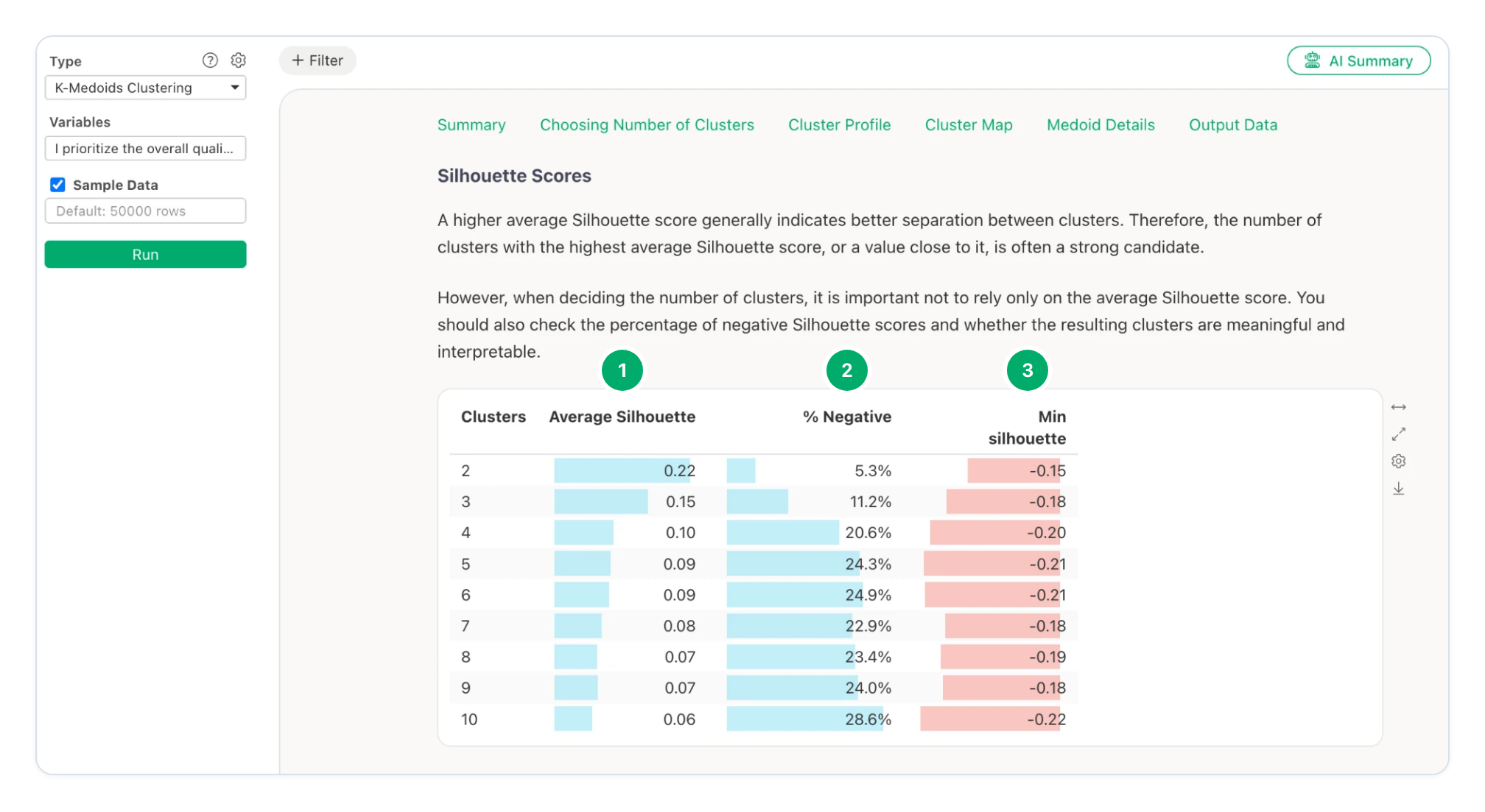
The Silhouette Scores table in Exploratory for 2 to 10 clusters, with the columns Average Silhouette, % Negative and Min silhouette.

Figure 10. Choosing Number of Clusters › Silhouette Scores for 2 to 10 clusters. Screenshot from Exploratory.

Average Silhouette. The mean silhouette score for each number of clusters. Here, 2 clusters have the highest score, 0.22.
% Negative. The percentage of respondents that are nearer to another cluster. It increases from 5.3% for 2 clusters to 28.6% for 10 clusters.
Min silhouette. The lowest silhouette score of one respondent for each number of clusters.

Note: Survey data often gives low silhouette scores, because the answers of different respondents overlap. Do not select the number of clusters from the score only. Here, 3 clusters have a lower score than 2 clusters (0.15 and 0.22), but the three clusters are easy to explain: price, quality and new products.

Read the report

After you click Run, Exploratory shows a report with six sections.

Report section	What it shows
Summary	The analysis conditions. For each cluster: rows, ratio, average and maximum distance to the medoid, medoid row ID and silhouette scores. Also the medoid values.
Choosing Number of Clusters	The silhouette scores, or the elbow curve and the reduction in variation.
Cluster Profile	Medoid values and averages by variable, the variables that characterize the clusters (η²), representative values and the variation in each cluster.
Cluster Map	The rows in two dimensions, calculated with PCoA from the clustering distances. Large points are the medoids.
Medoid Details	The medoid row of each cluster.
Output Data	Each row with its Cluster, Is Medoid, Distance to Medoid and Silhouette Score.

Keep the defaults first: Manhattan distance, Auto algorithm and standardized variables. Then use the silhouette scores to select the number of clusters.

Summary

K-medoids uses a real row, the medoid, as the center of each cluster.
PAM selects start medoids with BUILD. Then SWAP replaces medoids while the total distance decreases.
Outliers have a small effect on the medoids. Manhattan distance makes this effect even smaller.
Compare the silhouette scores, but select a number of clusters that you can explain.
For survey data on a Likert scale, each medoid is a real respondent with a possible answer pattern.

To try it, open Analytics in Exploratory and select Clustering Analysis › K-Medoids (Ordinal / Numerical).